1 Introduction
1.1 Preliminaries
Let us start by a general statement:
Another way of saying that is: Q.: “What is the chance of something happening?”
To answer this question we make use of Probability. Indeed, Probability is all about the certainty/uncertainty and the prediction of something happening. Some events are impossible, other events are certain to occur, while many are possible, but not certain to occur…
‘In this world there is nothing certain but death and taxes.’
Benjamin Franklin
1.2 Some examples
1.2.1 Example 1: SMI
The Swiss Market Index (SMI) is Switzerland’s blue-chip stock market index, which makes it the most followed in the country. Here below, a plot for the SMI index from 1-Jan-2020 to 31-Jan-2022 (about 530 observations).
Figure 1.1: We observe the index up to day t. Goal: prediction!!
For financial purposes, we may be interested in forecasting the value of the SMI for a time horizon of 60 days (about 2 months). We may use a fashionable tool, which is popular in machine learning, namely a neural network
Figure 1.2: What is the interpretation of the shadowed areas?
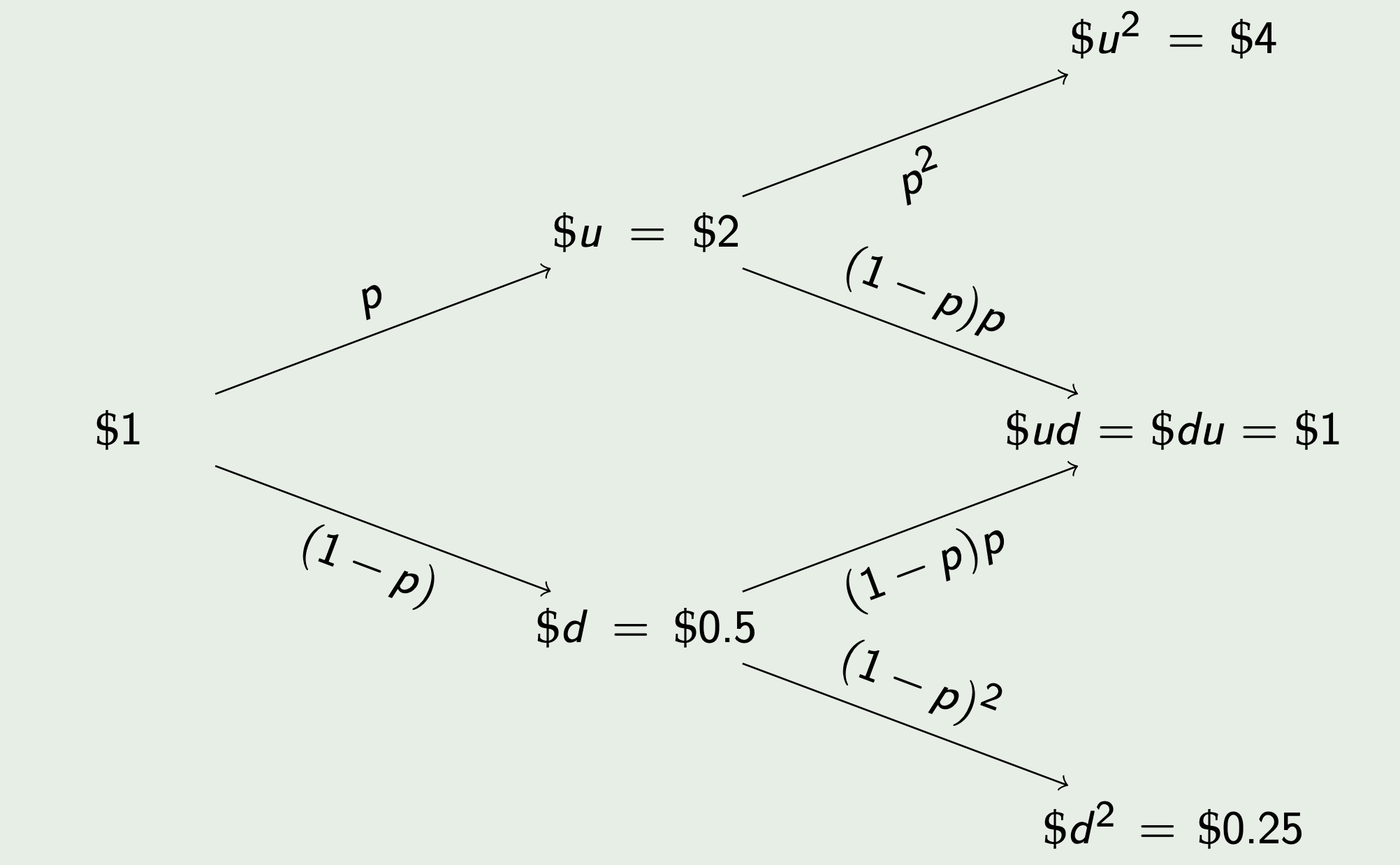
Let us imagine that we are going to model the uncertainty characterizing the SMI price by a simple model. With probability \(p=1 / 2\) the stock price moves up of a factor \(u\), and with probability \(1-p\) the price moves down of a factor \(d\). We denote the price at time \(t_{1}\) by \(u S_{0}\) if the price goes up, and by \(d S_{0}\) if the price goes down.
Let us set \(S_{0}=1 \$, u=2\) and \(d=1 / 2\). Can we say something about the price at time \(t_{2} ?\)
The price evolution is represented by a tree:
1.2.2 Example 2: Management
You work as data analyst in a large department store. You have records on the cash register receipts, over an extended period of time. From your data you find that
- \(30\%\) of the customers pay for their purchases by credit card,
- \(50\%\) pay by cash, and
- \(20\%\) pay by TWINT.
Question: Of the next 5 customers that make purchases at the store, what is the probability that 3 of them will pay by credit card?
Answer: Assume that how a customer pays for her purchases is the outcome of a Bernoulli trial with \(X_{i}=1\) if the customer pays by credit card, and \(X_{i}=0\) in case she pays with cash or TWINT. Given that the respective probabilities of these outcome are \(0.30\) and \(0.70\), and assuming that customers’ payment methods are independent of one another, it follows that
\[ X=\sum_{i=1}^{5} X_{i} \]
represents the number of customers that pay by credit card, and \(X\) has a binomial density function, with \(n=5\) and \(p=.3\) Therefore (see formula (3) in Lecture3-4.pdf)
\[ P(X=3)=\left(\begin{array}{l} 5 \\ 3 \end{array}\right) 0.3^{3}(1-0.3)^{5-3}=.1323 \]
1.2.3 Example 3: Quanta


Probability models are the basis for quantum physics: they characterize the uncertainty of properties of single energy “quanta” emitted by a ``perfect radiator" with a given temperature (\(T\)). Specifically, recall the famous Einstein’s equation \[\boxed{\mathcal{E} = m c^2}\] which expresses the energy \(\mathcal{E}\) in terms of the mass \(m\), a random quantity, and \(c\), the speed of light. Moreover, consider the geometric energy mean defined by \({\mathcal{E}_G} = c_0 k_B T\), where \(c_0 \approx 2.134\) and \(k_B\) is Boltzmann’s constant. Thus, one can define the random quantity
\[ W = \frac{\mathcal{E}}{{\mathcal{E}_G}}, \]
which is called quantum mass ratio.
The random behaviour of \(W\) can be described by a probability density function:
and for more links between quantum physics and probability:
1.3 What is Statistics/Probability?
In this course, we study Probability as a way to introduce Statistics.
Thus, we do not study Probability as a subject of interest in itself: we do not develop deep probability theory via measure theoretic arguments, rather we set up a few principles and methods which will be helpful for Statistics-the statistical analysis of time series, for the SMI case.
Question. Why is it important to study Probability/Statistics?
To understand why we must study Probability/Statistics, it is useful to first understand the answer to the following questions:
Question. What is Statistics? What is Probability?
Answer STATISTICS deals with the collection, presentation, analysis and interpretation of data in order to make rational decisions. Since, there is uncertainty in the data, we need PROBABILITY, which deals with uncertainty.
Aim and Scope
One makes use of Probability to develop methods to deal with uncertainty.Then, one applies these methods in tandem with Statistics to take decisions under uncertainty.
\(\leadsto\) Uncertainty is measured in units of probability, which is the currency of statistics. \(\leadsto\) Statistics is concerned with the study of data-driven decision making in the face of uncertainty.
1.4 A quick reminder of Mathematics
Probability theory is a mathematical tool. Hence, it is important to review some elemental concepts. Here are some of the formulae that we will use throughout the course.
1.4.1 Powers and Logarithms
- \(a^m \times a^n = a^{m+n}\);
- \((a^n)^m = a^{m \times n}\);
- \(\ln(\exp^{a}) = a\);
- \(a=\ln(\exp^{a}) = \ln(e^a)\);
- \(\ln(a^n) = n \times \ln a\);
- \(\ln (a \times b) = \ln (a) + \ln (b)\);
1.4.2 Differentiation
Derivatives will also play a pivotal role. Start by remembering some of the basic derivation operations:
Derivative of \(x\) to the power \(n\), \(f(x)= x^n\) \[\frac{d x^n}{dx} = n \cdot x^{n-1}\]
Derivative of the exponential function, \(f(x) = \exp(x)\) \[\frac{d \exp^{x}}{dx} = \exp^{x}\]
Derivative of the natural logarithm, \(f(x) = \ln(x)\) \[ \frac{d \ln({x})}{dx} = \frac{1}{x}\]
Moreover, we will make use of some fundamental derivation rules, such as:
1.4.3 Integration
Integrals will be crucial in many tasks. For instance, recall that integration is linear over the sum, i.e. \(\forall c, d \in \mathbb{R}\)
\[\int_{a}^{b} \left[c \times f(x) + d \times g(x) \right]dx = c \times \int_{a}^{b} f(x) dx + d \times \int_{a}^{b} g(x) dx; \]
- If the function is positive \(f(x) \geq 0, \forall x \in \mathbb{R}\), then its integral is also positive.
\[\int_{\mathbb{R}} f(x) dx \geq 0.\]
- For a continuous function \(f(x)\), the indefinite integral is
\[\int f(x) dx = F(x) + \text{const}\]
- while the definite integral is
\[F(b)-F(a)= \int_{a}^{b} f(x) dx, \quad b \geq a.\] And in both cases: \(f(x) = F'(x)\)
1.4.4 Sums
Besides integrals we are also going to use sums:
- Sums are denoted with a \(\Sigma\) operator and an index \(i\), as in:
\[\sum_{i=1}^{n} X_{i} = X_1 + X_2 +....+ X_n,\]
Moreover, for every \(\alpha_i \in \mathbb{R}\),
\[\sum_{i=1}^{n} \alpha_i X_{i} = \alpha_1 X_1 + \alpha_2 X_2 +....+ \alpha_n X_n;\]A double sum is a sum operated over two indices. For instance consider the sum of the product of two sequences \(\{x_1, \dots, x_n\}\) and \(\{y_1, \dots, y_m\}\),
\[\sum_{i=1}^{n} \sum_{j=1}^{m} x_{i}y_{j} = x_1y_1 + x_1 y_2 +... +x_2y_1+ x_2y_2 + \dots\]
- by carefully arranging the terms in the sum, we can establish the following identity:
1.4.5 Combinatorics
Finally, we will also rely on some combinatorial formulas. Specifically,
1.4.5.1 Factorial
\[ \begin{equation} n! = n \times (n-1) \times (n-2) \times \dots \times 1; \tag{1.1} \end{equation} \]
where \(0! =1\), by convention.
1.4.5.2 The Binomial Coefficient
The Binomial coefficient, for \(n \geq k\) is defined by the following ratio:
\[ \left(\begin{array}{l} n \\ k \end{array}\right)=\frac{n !}{k !(n-k) !}=C_{n}^{k} \]
which is helpful to express the Binomial Theorem \[ (x+y)^{n}=\left(\begin{array}{l} n \\ 0 \end{array}\right) x^{n} y^{0}+\left(\begin{array}{l} n \\ 1 \end{array}\right) x^{n-1} y^{1}+\cdots+\left(\begin{array}{c} n \\ n-1 \end{array}\right) x^{1} y^{n-1}+\left(\begin{array}{l} n \\ n \end{array}\right) x^{0} y^{n} \] or equivalently, making use of the sum notation, \[ (x+y)^{n}=\sum_{k=0}^{n}\left(\begin{array}{l} n \\ k \end{array}\right) x^{n-k} y^{k}=\sum_{k=0}^{n}\left(\begin{array}{l} n \\ k \end{array}\right) x^{k} y^{n-k} . \]
In English, the symbol \(\binom n k\) is read as “\(n\) choose \(k\).” We will see why in a few paragraphs.
Combinatorial formulas are very useful when studying permutations and combinations both very recurrent concepts.
Permutations
A permutation is an ordered rearrangement of the elements of a set.
Example 1.1 (Three friends and three chairs) Suppose we have three friends Aline (\(A\)), Bridget (\(B\)) and Carmen (\(C\)) that want to sit on three chairs during lunchtime.
- One day, you see Aline on the left, Bridget in the center and Carmen on the right, i.e. \((A, B, C)\)
- The next day, Bridget sits first, Aline second and Carmen right, i.e. \((B, A, C)\)
These rearrangements constitute two Permutations of the set of three friends \(\{A, B, C\}\).
You then start wondering in how many ways these three friends can sit. With such a small set, it is easy to take a pen and some paper to write down all the possible permutations:
\[(A, B, C), (A, C, B), (B, A, C), (B, C, A), (C, A, B), (C, B, A)\]
As you can see, the total number of permutations is : \(N = 6.\) But also \(6= 3 \times 2 \times 1 = 3!\). This is by no means a coincidence. To see in detail why let us consider each chair as an “experiment” and its occupant an “outcome.”
- Chair (Experiment) 1 : has 3 possible occupants (outcomes): {\(A\), \(B\), \(C\)}.
- Chair (Experiment) 2 : has 2 possible occupants (outcomes): either \(\{B,C\}\), \(\{A,C\}\) or \(\{A,B\}\)
- Chair (Experiment) 3 : has 1 possible occupant (outcomes) : \(\{A\}\), \(\{B\}\) or \(\{C\}\)
Here, we can apply the Fundamental Counting Principle, i.e. from Ross (2014):
If \(r\) experiments that are to be performed are such that the first one may result in any of \(n_1\) possible outcomes; and if, for each of these \(n_1\) possible outcomes, there are \(n_2\) possible outcomes of the second experiment; and if, for each of the possible outcomes of the first two experiments, there are \(n_3\) possible outcomes of the third experiment; and so on, then there is a total of \(n_1 \times n_2 \times \cdots \times n_r\) possible outcomes of the \(r\) experiments.
Hence: \(3 \times 2 \times 1 = 3! = 6\)
Definition 1.2 Permutations help you answer the question: How many different ways can we arrange \(n\) objects?
- In the 1st place: \(n\) possibilities
- In the 2nd place: \((n-1)\) possibilities
- …
- Finally, \(1\) possibility
- A gorgeous sunflower 🌻
- An old-timey Radio 📻
- A best-selling book 📖
- An elegant pen 🖊
- An incredibly charismatic turtle 🐢
In how many ways can you arrange them on the shelf?
Let us use this Exercise to go further. Suppose now that the shelf is now a bit more narrow, and you can only show 3 products instead of 5. How many ways can we select \(3\) items among the \(5\)?
By the Fundamental Counting Principle you have \(5\times4\times3\) ways of selecting a the 3 elements. If we write them in factorial notation, this represents \[ 5\times4\times3 = \frac{5\times4\times3\times2\times1}{2\times1} = \frac{5!}{2!} = \frac{5!}{(5-3)!} \] This formula can be interpreted as follows:
If you select \(3\) presents from the list, then you have \((5-3)\) other presents that you won’t select. The latter set has \((5-3)!\) possibilities which have to be factored out from the \(5!\) possible permutations.
As you can see, we are slowly but surely arriving to the definition of \(\binom n k\) in (??). However, there is still one more element…
Combinations
Implicit in this example, is the notion that the order in which these elements are displayed is important. This means, that the set (🌻, 📖, 🐢) is different from the set ( 📖, 🐢, 🌻) which, as you can assess, is a permutation of the original draw.
Let us suppose that the order is not important. This implies that once the 3 gifts are chosen all the permutations of this subset are deemed equivalent. Hence, the subset (🌻, 📖, 🐢), is deemed equivalent as all its \(3! = 6\) permutations and we have to factor out this amount from the previous result, by dividing the \(3!\) different ways you can order the selected presents.
If we put this in a formula, we have \[\frac{5!/(5-3)!}{3!}\] ways to select the \(3\) presents:
\[\frac{5!/(5-3)!}{3!}= \frac{5!}{3!2!} = \binom 5 3 = C_5^3.\] This gives you the total number of possible ways to select the \(3\) presents when the order does not matter. There are thus "\(5\) choose \(k\)" ways of choosing 3 elements among 5.
In general, \(n \choose k\) results from the following computations.
In the 1st place: \(n\)
In the 2nd place: \((n-1)\)
…
In the \(k\)-th place: \((n-k+1)\)
We have \(k!\) ways to permute the \(k\) objects that we selected
The number of possibilities (without considering the order) is:
\[\frac{n!/(n-k)!}{k!} = \frac{n!}{k!(n-k)!}{\color{gray}{=C^{k}_n}}\]
For the Problem Set \(2\), you will have to make use of \(C^{k}_n\) in Ex2-Ex3-Ex5. Indeed, to compute the probability for an event \(E\), will have to make use of the formula:
\[\begin{equation} P(E)=\dfrac{\text{number of cases in E}}{\text{number of possible cases}}. \tag{1.2} \end{equation}\]This is a first intuitive definition of probability, which we will justify in the next chapter. For the time being, let us say that the combinatorial calculus will be needed to express both the quantities (numerator and denominator) in (1.2).
The name “Binomial Coefficient” is closely associated with the Binomial Theorem, which provides the expression for the power \(n\) of the sum of two variables \((x+y)\) as a sum:
Theorem 1.1 (Binomial Theorem - Pascal 1654) For \(n=0,1, 2,\dots\), we have:
\[(x+y)^n = {n \choose 0}x^n y^0 + {n \choose 1}x^{n-1}y^1 + \cdots + {n \choose n-1}x^1 y^{n-1} + {n \choose n}x^0 y^n;\]
The sum is finite and stops after n+1 terms.Equivalently, making use of the sum notation,
\[(x+y)^n = \sum_{k=0}^n {n \choose k}x^{n-k}y^k = \sum_{k=0}^n {n \choose k}x^{k}y^{n-k}.\]
Example 1.2 Let us compute the binomial coefficients for polynomials of different degrees \(n\):
- for \(n=1\)
\[\begin{align} (x+y)^1 &= {1 \choose 0}x^1 y^0 + {1 \choose 1}x^0 y^{1}\\ &= x + y \end{align}\]
- for \(n=2\) we have
\[\begin{align} (x+y)^2 &= {2 \choose 0}x^2 y^0 + {2 \choose 1}x^{1}y^1 + {2 \choose 2}x^0 y^{2} \\ &= x^2 + 2 x y + y^{2} \end{align}\]
- for \(n=3\) we have \[\begin{align} (x+y)^3 &= {3 \choose 0}x^3 y^0 + {3 \choose 1}x^{2}y^1 + \cdots + {3 \choose 2}x^1 y^{2} + {3 \choose 3}x^0 y^3 \\ &= y^3 + 3xy^2 + 3x^2y+x^3 \end{align}\]
1.4.6 Limits
The study of limits will be crucial in many tasks:
- The limit of a finite sum is an infinite series: \[\lim_{n \to \infty} \sum_{i=1}^n x_i = \sum_{i=1 }^\infty x_i \nonumber\]
- The Exponential function, characterised as a limit: \[ e^x = \lim_{n \rightarrow \infty} \left(1 + \frac{x}{n}\right)^n \nonumber\]
- The Limit of a Negative Exponential function: Let \(\alpha >0\) \[\lim_{x \to \infty} {\alpha e^{-\alpha x}} = 0 \nonumber\]
- The Exponential function, characterised as an infinite series: \[e^x = \sum_{i = 0}^{\infty} {x^i \over i!} = 1 + x + {x^2 \over 2!} + {x^3 \over 3!} + {x^4 \over 4!} + \dots\]