Chapter 6 Simple Models in JAGS
6.1 Revisiting Hierarchical Structures
6.1.1 What is a hierarchical model?
Parent and Rivot (2012): A model with three basic levels
- A data level that specifies the probability distribution of the observables at hand given the parameters and the underlying processes
- A latent process level depicting the various hidden ecological mechanisms that make sense of the data
- A parameter level identifying the fixed quantities that would be suficient, were they known, to mimic the behavior of the system and to produce new data statistically similar to the ones already collected
Also
- Observation model: distribution of data given parameters
- Structural model: distribution of parameters, governed by hyperparameters
- Hyperparameter model: parameters on priors
Other Definitions
- “Estimating the population distribution of unobserved parameters” (Gelman et al. 2013)
- “Sharing statistical strength”: we can make inferences about data-poor groups using the entire ensemble of data
- Pooling (partially) across groups to obtain more reliable estimates for each group
6.1.2 Hierarchical Model Example
“Similar, but not identical” can be shown to be mathematically equivalent to assuming that unit-specific parameters, \(\theta_i, i = 1,...,N\), arise from a common “population” distribution whose parameters are unknown (but assigned appropriate prior distributions)
\[\theta_i \sim N(\mu,\sigma_2)\]
\[\mu \sim N(.,.); \sigma \sim unif(.,.)\]
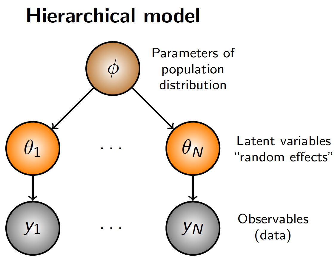
We learn about \(\theta_i\) not only directly through \(y_i\), but also indirectly through information from the other \(y_j\) via the population distribution parameterized by \(\phi\)
Example: A normal-normal mixture model
- Let \(y_i=(y_{i1}, y_{i2},...y_{in})\) denote replicate measurements made on each of \(j=1,2,...n\) subjects
- Observation model: \(y_{ij}\sim N(\alpha_j,\sigma^2)\)
- \(y_{ij}\) is assumed normally-distributed with a mean that depends on a subject-specific parameter, \(\alpha_j\)
- Assume that \(\alpha_j\)’s come from a common population distribution \(\alpha_{j}\sim N(\mu,\sigma_\alpha^2)\)
Ecological data are characterized by: - Observations measured at multiple spatial and/or temporal scales - An uneven number of observations measured for any given subject or group of interest (i.e., unbalanced designs) - Observations that lack independence (i.e., the value of a measurement at one location or time period influences the value of another measurement made at a different location or time period - Widely applicable to many (most) ecological investigations
Desirable properties of hierarchical models 1. Accommodate lack of statistical independence 2. Scope of inference 3. Quantify and model variability at multiple levels 4. Ability to “borrow strength” from the entire ensemble of data (phenomenon referred to as shrinkage)
6.1.3 Borrowing Strength?
- Make use of all available information
- Results in estimators that are a weighted composite of information from an individual group (e.g., species, individual, reservoir, etc.) and the relationships that exist in the overall sample
- Could fit separate ordinary least squares (OLS) regressions to each group (e.g., reservoir) and obtain estimate of a slope and intercept
- OLS will give estimates of parameters, however, they may not be very accurate for any given group
- Depends on sample size within a group (\(n_j\)) and the range represented in the level-1 predictor variable, \(X_{ij}\)
- If \(n_j\) is small then intercept estimate will be imprecise
- If sample size is small or a restricted range of \(X\), the slope estimate will be imprecise
Hierarchical models allow for taking into account the imprecision of OLS estimates
- More weight to the grand mean when there are few observations within a group and when the group variability is large compared to the between-group variability
- E.g., small sample size for a given group = not very precise OLS estimate, so value “shrunk” towards population mean
- More weight is given to the observed groups mean if the opposite is true
- Thus, hierarchical models accounts and allows for the smallsample sizes observed in some groups
- Same is true for the range represented in predictor variables (i.e.., hierarchical models accounts and allows for the small and limited ranges of \(X\) observed in some groups)
6.1.4 Shrinkage toward the grand mean (\(\mu_\alpha\))
The estimate of \(\alpha_j\) is a linear combination of the population-average estimate \(\mu_\alpha\) and the ordinary least squares (OLS) estimate, \(\alpha^{OLS}\)
\[\alpha_j = w_j \times \alpha^{OLS} + (1-w_j) \times \mu_\alpha\]
The weight, \(w_j\) is a ratio of the between group variability (\(\sigma_{\alpha}^2\)) to the sum of the within and between-group variability (i.e., total variability)
\[w_j=\frac{n_j \times \sigma_{\alpha}^2}{n_j \times \sigma_{\alpha}^2 +\sigma^2}\]
where \(n_j=\) sample size
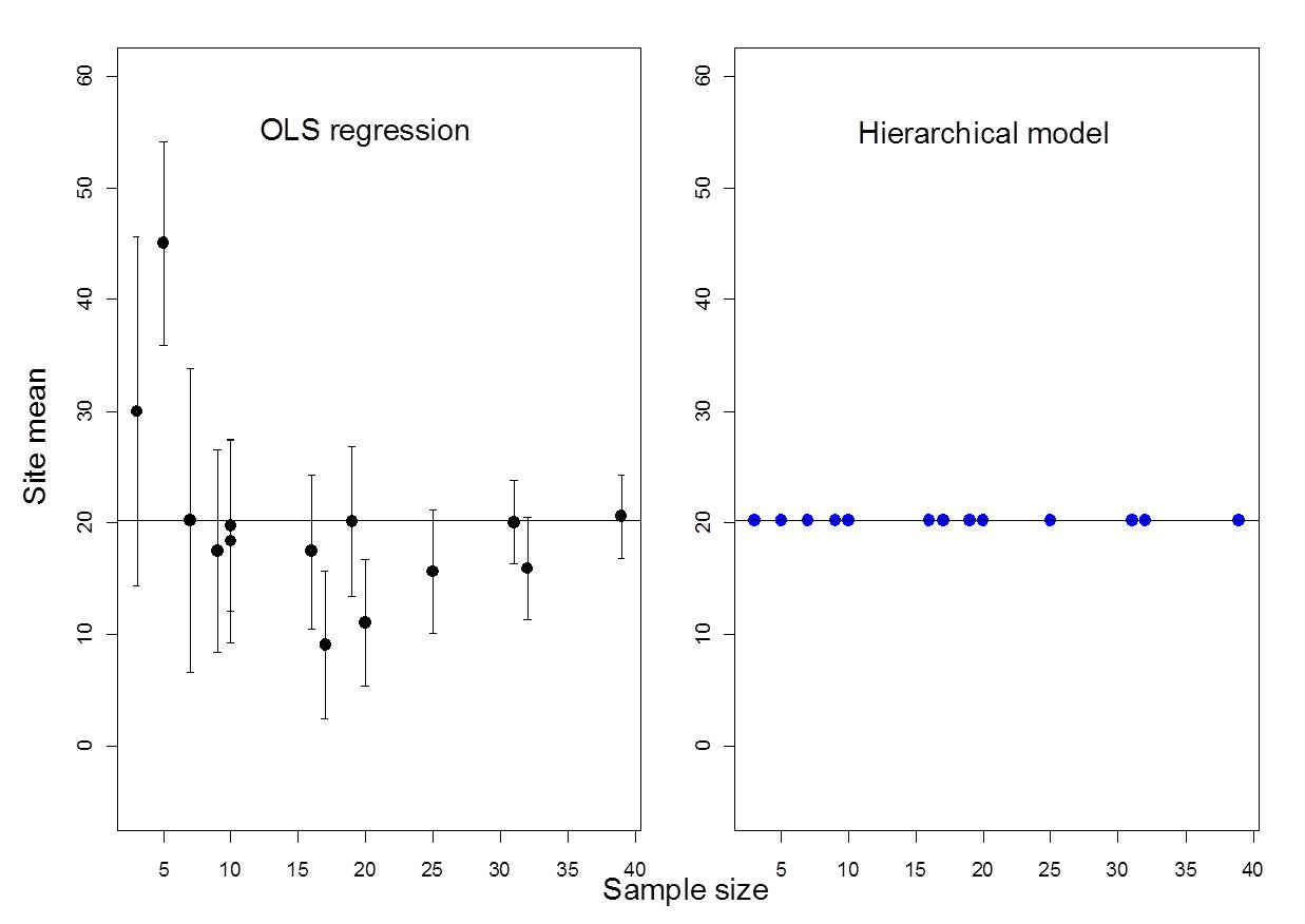
Figure 6.1: Example where ICC = 0% (i.e., no among-group variability)
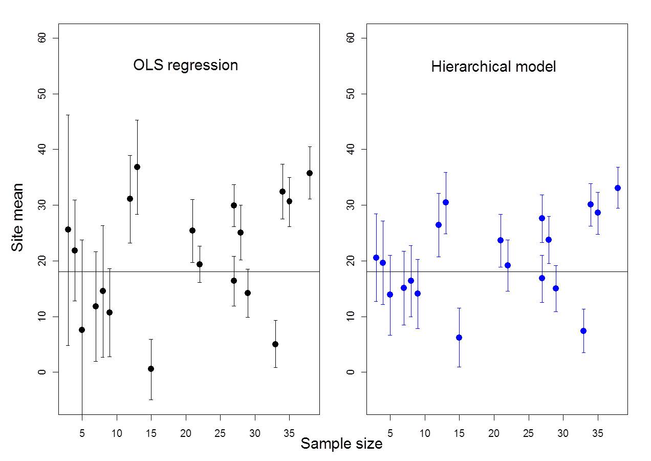
Figure 6.2: Example where ICC = 13%
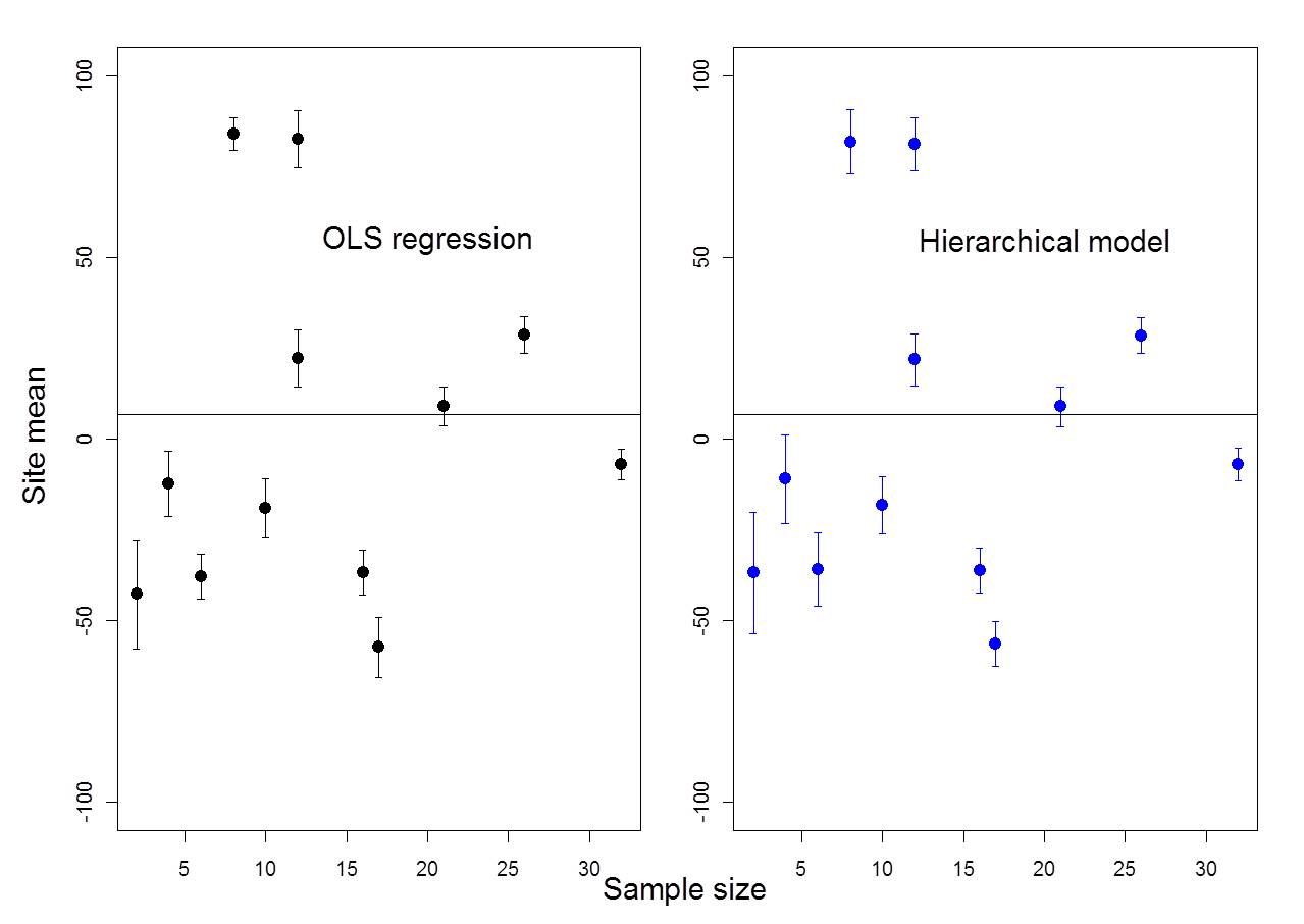
Figure 6.3: Example where ICC = 80%
6.2 Simple Linear Regression
The model from a Bayesian point of view
\[y_i \sim N(\alpha + \beta x_i, \sigma^2)\]
for \(i, ...n\)
Priors: \[\alpha \sim N(0, 0.001)\] \[\beta \sim N(0, 0.001)\] \[sigma\sim U(0, 10)\]
6.2.1 Varying Coefficient Models
Few people run models in JAGS because they want fixed effects, and in fact, because parameters need to have an underlying distribution you will have the option to create random effects, or varying coefficients, very easily. Before we start on the different types of simple varying coefficient models, let’s visually review them.
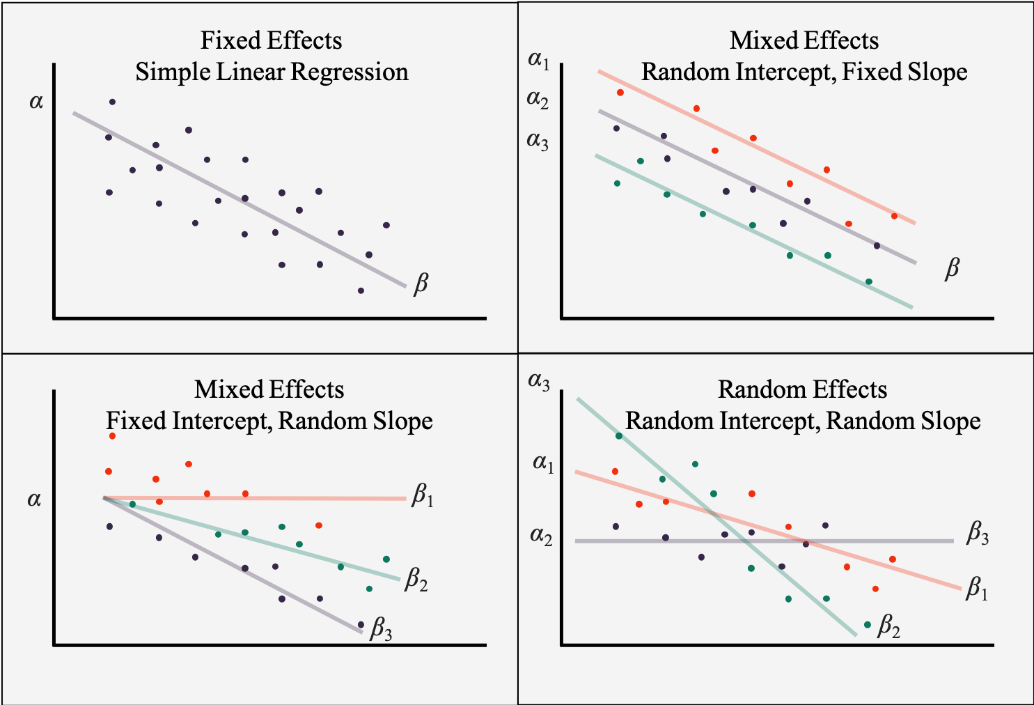
Figure 6.4: Examples of different varying coefficient models
6.3 Varying Intercept Model
Another way of labeling a varying intercept model is a one-way ANOVA with a random effect. A one-way ANOVA is among the simpler of statistical models, and a little complexity has been added by changing the single fixed factor to be random. Either terminology is accurate and acceptable, but because ANOVAs model means and means without slopes are intercepts, we will often hear an ANOVA called an \(intercepts model\), with the modifier varying meaning that group levels are random and can vary from the grand mean.
Let’s think about the varying intercepts model with an example.
Say we have multiple measurements of total phosphorus (\(TP\)) taken from \(i\) lakes located in \(j\) regions (\(j=1,2,...J\)). The number of lakes sampled in each region varies, and we want to estimate the mean \(TP\) for each region. We can assign each region its own intercept (i.e., it’s own mean \(TP\)) and we will allow these intercepts to come from a normal distribution characterized by an overall mean \(TP\) (\(\mu_\alpha\)) and between-region variance (\(\sigma_{\alpha}^2\)).
The model can be expressed as follows:
\[y_i \sim N(\alpha_{j(i)}, \sigma^2)\]
for \(i, ...n\)
\[\alpha_j \sim N(\mu_{\alpha}, \sigma_{\alpha}^2)\] for \(j,...J\)
\[\mu_{\alpha} \sim N(0, 0.001)\] \[\sigma_{\alpha}^2 \sim U(0, 10)\] \[\sigma\sim U(0, 10)\]
# Likelihood
for(i in 1:n){
  y[i] ~ dnorm(mu[i], tau)
  mu[i] <- alpha[group[i]]
}

for(j in 1:J){}
alpha[j] ~ dnorm(mu.alpha, tau.alpha)
}

# Priors
mu.alpha ~ dnorm(0,0.001)
sigma ~ dunif(0,10)
sigma.alpha ~ dunif(0,10)

# Derived quantities
tau <- pow(sigma,-2)
tau.alpha <- pow(sigma.alpha,-2)
6.3.1 Nested Indexing
In random intercept models we have observation \(i\) in region \(j\). Multiple \(i\)’s can be observed within a single \(j\). Therefore, we have multiple observations per some grouping variable, so we have two indexes, \(i\) and \(j\). Up until this point, we only had observation \(i\), which was easily accommodated in a single for loop. “Nested indexing” is a way of accommodating this type of data structure
6.3.2 Intraclass correlation coefficient (ICC)
This is another version of the one-way ANOVA with a random effect. The primary difference between this and the model above is that here we are going to actually calcuate the Intraclass correlation coefficient, \(ICC\), as a derived quantity, in order to help us understand more about where the variability is in the data.
Recall that \(ICC\) is a measure of the variability within groups compared to among groups.
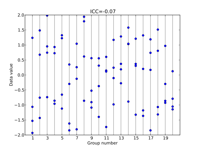
Figure 6.5: Low ICC
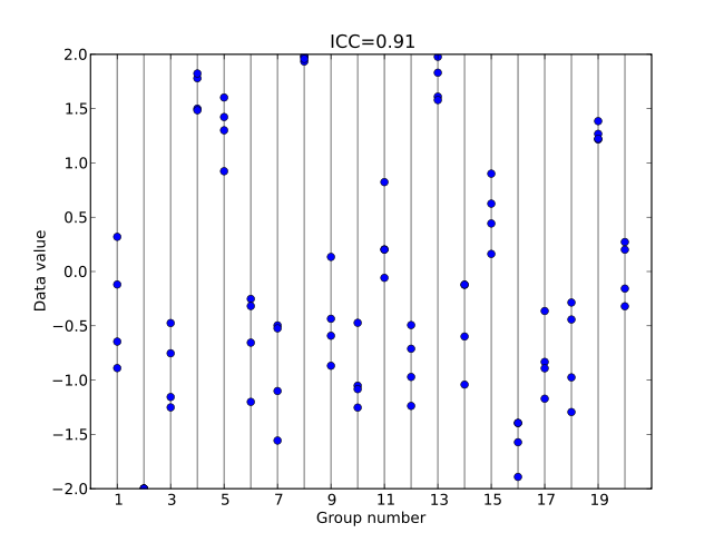
Figure 6.6: High ICC
The model can be expressed the same way as the one-way ANOVA with a random effect:
\[y_i \sim N(\alpha_{j(i)}, \sigma^2)\] for \(i, ...n\)
\[\alpha_j \sim N(\mu_{\alpha}, \sigma_{\alpha}^2)\] for \(j,...J\)
Recall that the total variance \(= \sigma^2 + \sigma_{\alpha}^2\) and therefore
\[ICC = \frac{\sigma_{\alpha}^2}{\sigma^2 + \sigma_{\alpha}^2}\] Both terms required in the ICC equation are already being estimated by the model, so this is a good example of a derived quantity.
6.3.3 Varying Intercept, Fixed Slope Model
We can easily add a level-1 covariate (slope) to our model, but because it is not varying, it will create a model where the effect of the covariate is equal on all groups, although the intercept of the groups may vary among groups.
This model might look like:
\[y_i \sim N(\alpha_{j(i)} + \beta x_i, \sigma^2)\]
for \(i, ...n\)
\[\alpha_j \sim N(\mu_{\alpha}, \sigma_{\alpha}^2)\]
for \(j,...J\)
Note that the second level model (the model for \(\alpha_j\)’s) is the same as the previous model. The only change is that we have added an \(x\) predictor and a \(\beta\) that represents a single, common slope, or the effect of \(x\) on \(y\). Although \(\beta\) is not varying, we still need to give it a prior, because it is an estimated parameter and not a deterministic node.
\[\mu_{\alpha} \sim N(0, 0.001)\]
\[\beta \sim N(0,0.0001)\] \[\sigma_{\alpha}^2 \sim U(0, 10)\] \[\sigma\sim U(0, 10)\]
6.4 Varying Slope Model
A single slope may make sense in some applications where the change in a covariate effects all groups the same, despite the fact that the groups may start at different values. However, there is a good chance that covariates hold the potential to have different directions and magnitudes of an effect on different groups. In cases like this, a varying slope would make sense. In ecology, the assumption that many processes are spatially and/or temporally homogeneous or invariant may not be valid. For example, spatial variation in the a stressor-response relationship may vary depending on local landscape features.
Another important attribute of varying slopes is that they can help avoid Simpson’s Paradox, which is when a trend appears in several different groups of data but disappears or reverses when these groups are combined.
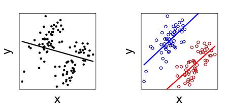
Figure 6.7: Example of Simpson’s Paradox

Figure 6.8: Most quantitative ecologists cannot resist the temptation to include a cartoon of Homer Simpson when referencing Simpson’s Paradox.
Recall our varying intercept model, and we will change one thing in the (level-1) equation. We will index \(\beta\) by \(i\) and \(j\) in the same way we did for \(\alpha\) in the varying intercept model.
\[y_i \sim N(\alpha_{j(i)} + \beta_{j(i)} x_i, \sigma^2)\] for \(i, ...n\)
The second level of our model changes more dramatically, because we now have two varying coefficient and need to model both their variances and their correlation.
\[\left(\begin{array} {c} \alpha_j\\ \beta_j \end{array}\right) \sim N \left(\left(\begin{array} {c} \mu_{\alpha}\\ \mu_{\beta} \end{array}\right), \left(\begin{array} {cc} \sigma_{\alpha}^2 & \rho\sigma_{\alpha}\sigma_{\beta}\\ \rho\sigma_{\alpha}\sigma_{\beta} & \sigma_{\beta}^2 \end{array}\right) \right)\]
for \(j,...J\)
Several of these terms we have seen before, specifically the terms involving \(\alpha\), the intercept. However, many of the \(\beta\) terms are used similarly to the \(\alpha\) terms. After understanding that the equation is written in matrix-notation to accomdate both varying parameters, see that the row for \(\beta_j\) contains the mean \(\beta\)’s, expressed as a mean, \(\mu_{beta}\). The final part is the variance-covariance matrix, which might be simpler that it appears. Note that we have already recoginized \(\sigma_{\alpha}\) as the among-group variance for intercepts, and \(\sigma_{\beta}\) is simple the among-group variance for slopes. The only term remaining is the one involving \(\sigma_{\alpha\beta}\), which represents the joint variability of \(\alpha_j\) and \(\beta_j\). Perhaps the important part of this term is that it is prefaced with \(\rho\), the Greek symbol commonly used for correlation. So the term \(\rho\sigma_{\alpha}\sigma_{\beta}\) is quantifying the correlation between the varying parameters, which is important to know because we want and need the correlation to be minimal.
Finally, we need priors for the model. Again, think about building on previous models that we have learned. This is not entirely a new model, so use what you already know, and add the new parts.
\[\mu_{\alpha} \sim N(0,0.001)\]
\[\mu_{\beta} \sim N(0,0.001)\]
\[\sigma\sim U(0, 10)\]
\[\sigma_{\alpha} \sim U(0, 10)\] \[\sigma_{\beta} \sim U(0, 10)\] \[\rho \sim U(-1, 1)\]
Note that ICC cannot be applied to this model for reasons we won’t get into.
6.4.1 Correlation between parameters
When estimated parameters are correlated, it may be a sign of model fitting problems. Correlated parameters may mean that the parameters are not able to independently explore parameter space, which may lead to poor estimates. Additionally, if the estimates are reliable but the parameters are correlated, it may mean that you aren’t getting much information from the data that are correlated. Regardless, correlated parameters are a problem in your models and need to be addressed. (Also, there is not agreed upon threshold for “highly correlated”, but by the time correlations approach 0.7, you may want to start looking into things.)
Fortunatly, there are several (and mostly simple) things to do to address parameter correlation. The best thing to do is often to center and/or standardize your model covariates, which has been discussed before. Standardizing data typically reduces correlation between parameters, improves convergence, may improve parameter interpretation, and can also mean that the same priors can be used.
Going back to the PLD data that we have examined, note that the correlation of intercepts and effect of temperature based on the raw data is high, at about -0.95.
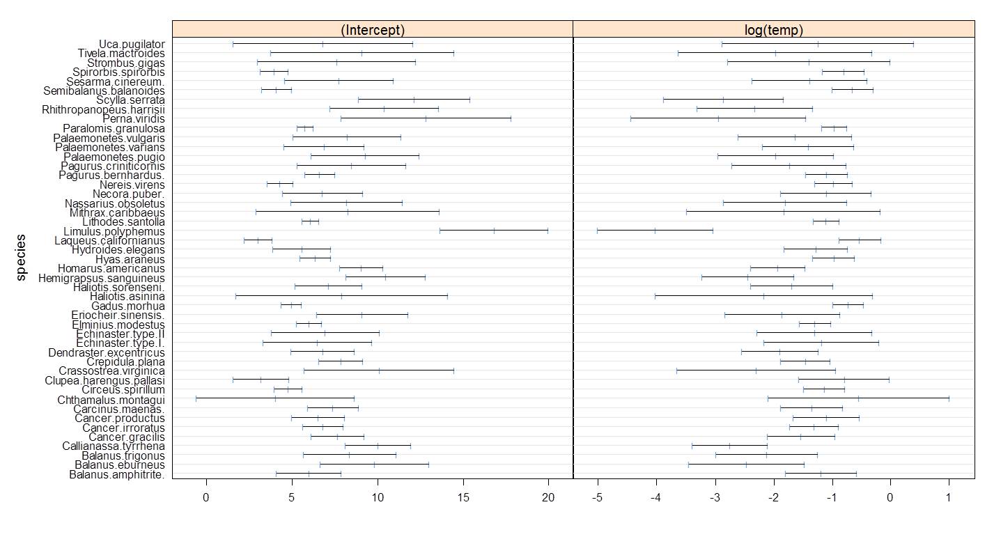
Figure 6.9: Correlation between intercepts and effect of log(temperature) for the raw PLD dataset. Correlation is around 0.95.
In the PLD paper, a centering constant was used that greatly reduced the correlation.
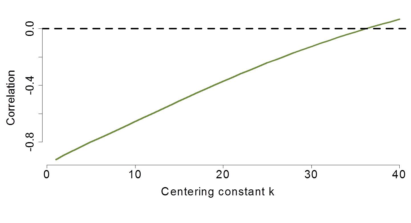
Figure 6.10: Simulation of varying centering constants examined to reduce parameter correlation.
The centering of the temperature by -15 resulted in near elimination of the parameter correlation. Note that this example is about as impressive as you might find and you should not expect results this dramatic in all data. However, centering and/or standardizing does routinely reduce correlation as advertised.
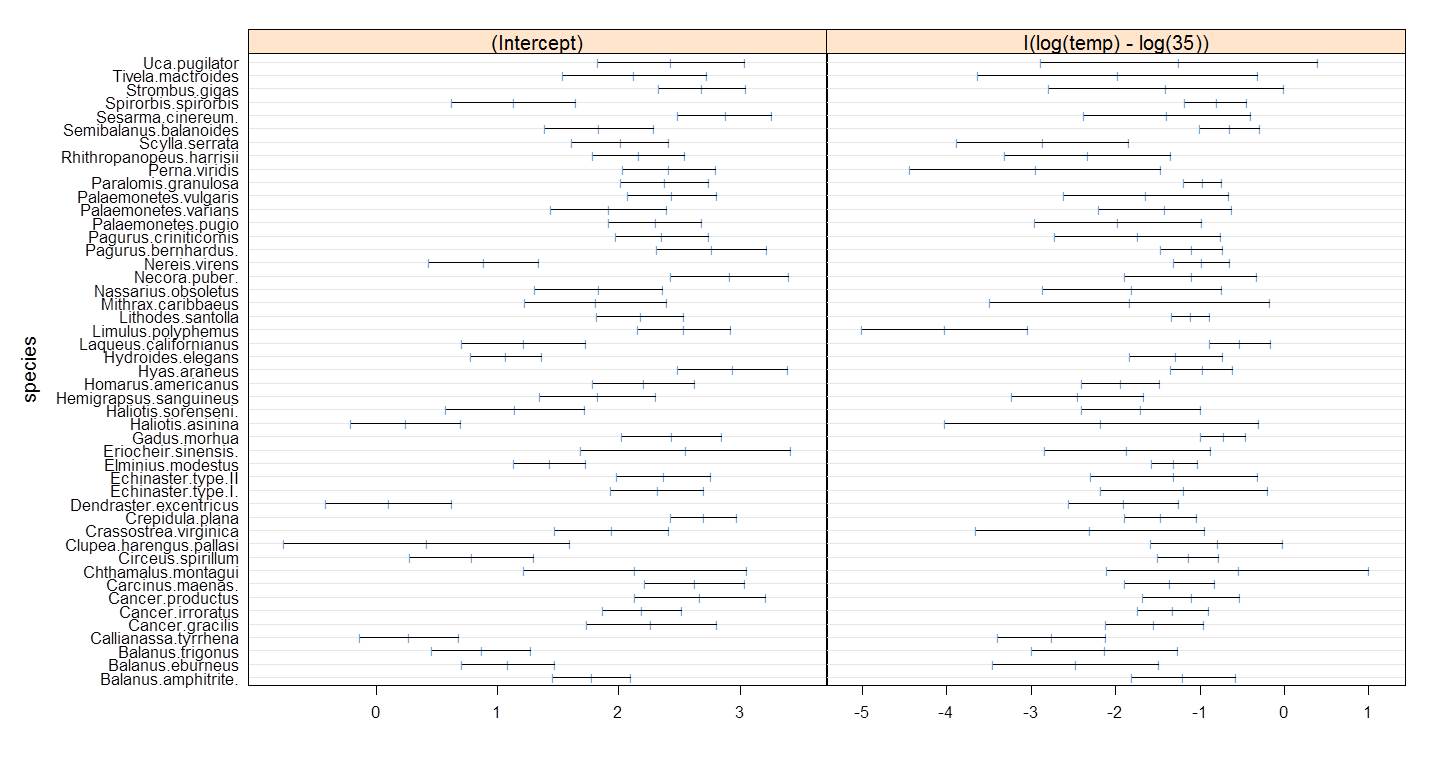
Figure 6.11: PLD intercepts and slopes with almost no correlation.
Recall that centering changes the values, but not the scale of the data. Think about it as shifting the numberline under your data. Mean-centering is also a very common type of centering. Standardizing your data changes both the values and the scale. There is a reasonable literature on various standardizing approaches, but mean-centering and dividing by 1 or 2 standard deviations are very common and usually produce good results.
6.4.2 Correlation between 2 or more varying parameters
Another way to represent the models with 2 or more varying parameters is:
\[y_i \sim N(X_i B_{j(i)}, \sigma^2)\] for \(i, ...n\)
\[B_i \sim N(M_B, \Sigma_B)\] for \(j,...J\)
Where \(B\) represents the matrix of group-level coefficients, \(M_B\) represents the population average coefficients (i.e., the mean of the distributions of the intercepts and slopes), and \(\Sigma_b\) represents the covariance matrix.
Once we move beyond 2 varying parameters, it is no longer possible to set diffuse priors one parameter at a time; each correlation is restricted to be within -1 and 1 and correlations are jointly constrained. In other words, we need to put a prior on the covariance matrix (\(\Sigma_B\)) itself.
To accomplish this “prior on a matrix”, we will use the scaled inverse-Wishert distribution. This distribution implies a uniform distribution on the correlation parameters. According to Gelman and Hill (2006), “When the number \(K\) of varying coefficients per group is more than two, modeling the correlation parameters \(\rho\) is a challenge.” But the scaled inverse-Wishert appraoch is a “useful trick”. Note that Kéry (2010) does not go so far as to deal with this issue. While this adds some model complexity, ultimtely this development is something that will be provided in the JAGS model code and never really changed. Note that this distribution requires the library MCMCpack.
Below is an example of coding for 2 varying coefficients without using the Wishert distribution. This approach will work, but is not recommended.
#### Dealing with variance-covariance of random slopes and intercepts
# Convert covariance matrix to precision for use in bivariate normal
  Tau.B[1:K,1:K] <- inverse(Sigma.B[,])

# variance among intercepts
  Sigma.B[1,1] <- pow(sigma.a, 2)
  sigma.a ~ dunif (0, 100)

# Variance among slopes
  Sigma.B[2,2] <- pow(sigma.b, 2)
  sigma.b ~ dunif (0, 100)

# Covariance between alpha's and beta's
  Sigma.B[1,2] <- rho * sigma.a * sigma.b
  Sigma.B[2,1] <- Sigma.B[1,2]

# Uniform prior on correlation
  rho ~ dunif (-1, 1)
Below is code for the model variance-covariance using the Wishert distribution. There are computational advantages to this, in addition to the fact that it easily scales up for more than 2 varying coefficients.
References
Gelman, Andrew, John B Carlin, Hal S Stern, David B Dunson, Aki Vehtari, and Donald B Rubin. 2013. Bayesian Data Analysis. Chapman; Hall/CRC.
Gelman, Andrew, and Jennifer Hill. 2006. Data Analysis Using Regression and Multilevel/Hierarchical Models. Cambridge university press.
Kéry, Marc. 2010. Introduction to Winbugs for Ecologists: Bayesian Approach to Regression, Anova, Mixed Models and Related Analyses. Academic Press.
Parent, Eric, and Etienne Rivot. 2012. Introduction to Hierarchical Bayesian Modeling for Ecological Data. Chapman; Hall/CRC.