Chapter 4 Bayesian Machinery
4.1 Bayes’ Rule
\[P(\theta|y)=\frac{P(y|\theta)\times P(\theta)}{P(y)}\] where
- \(P(\theta|y)\) = posterior distribution
- \(P(y|\theta)\) = Likelihood function
- \(P(\theta)\) = Prior distribution
- \(P(y)\) = Normalizing constant
4.1.1 Posterior Distribution: \(p(\theta | y)\)
The posterior distribution (often abbreviated as the posterior) is simply the way of saying the result of computing Bayes’ Rule for a set of data and parameters. Because we don’t get point estimates for answers, we correctly call it a distribution, and we add the term posterior because this is the distrution produced at the end. You can think of the posterior as a astatement about the probability of the parameter value given the data you observed.
“Reallocation of credibilities across possibilities.” - John Kruschke
4.1.2 Likelihood Function: \(p(y | \theta)\)
- Skip the math
- Consider it similar to other likelihood functions
- In fact, it will give you the same answer as ML estimator (interpretation differs)
4.2 Priors: \(p(\theta)\)

Figure 4.1: Prior information can be useful.
- Distribution we give to a parameter before computation
- WARNING: This is historically a big deal among statisticians, and subjectivity is a main concern cited by Frequentists
- Priors can have very little, if any, influence (e.g., diffuse, vague, non-informative, unspecified, etc), yet all priors are technically informative.
- Much of ecology uses diffuse priors, so little concern
- But priors can be practical if you really do know information (e.g., even basic information, like populations can’t be negative values)
- Simple models may not need informative priors; complex models may need priors
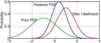
Figure 4.2: Example of prior, likelihood, and poserior distributions.
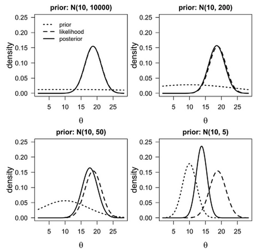
Figure 4.3: Example of prior influence based on prior parameters.
You may not use informative priors when starting to model. Regardless, always think about your priors, explore how they work, and be prepared to defend them to reviewers and other peers.
“So far there are only few articles in ecological journals that have actually used this asset of Bayesian statistics.” - Marc Kery (2010)
4.3 Normalizing Constant: \(P(y)\)
The normalizing constant is a function that converts the area under the curve to 1. While this may seem technical—and it is—this is what allows us to interpret Bayesian output probabilistically. The normalizing constant is a high dimension integral that in most cases cannot be analytically solved. But we need it, so we have to simulate it. To do this, we use Markov Chain Monte Carlo, MCMC.
4.3.1 MCMC Background
- Stan Ulam: Manhattan project scientist
- The solitaire problem: How do you know the chance of winning?
- Can’t really solve… too much complexity
- But we can automate a bunch of games and monitor the results—basically we can do something so much that we assume the simulations are approximating the real thing.
Fun Fact: There are 80,000,000,000,000,000,000,000,000,000,000,000,000,000,000,000,000, 000,000,000,000,000,000 solitaire combinations!
Markov Chain: transitions from one state to another (dependency) Monte Carlo: chance applied to the transition (randomness)
- MCMC is a group of functions, governed by specific algorithms
- Metropolis-Hastings algorithm: one of the first algorithms
- Gibbs algorithm: splits multidimensional \(\theta\) into separate blocks, reducing dimensionality
- Consider MCMC a black box, if that’s easier
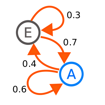
Figure 4.4: MCMC samplers are designed to sample parameter space with a combination of dependency and randomness.
4.3.2 MCMC Example
A politician on a chain of islands wants to spend time on each island proportional to each island’s population.
- After visiting one island, she needs to decide…
- stay on current island
- move to island to the west
- move to island to the east
But she doesn’t know overall population—can ask current islanders their population and population of adjacent islands
- Flips a coin to decide east or west island
- if selected island has larger population, she goes
- if selected island has smaller population, she goes probabilistically
MCMC is a set of techniques to simulate draws from the posterior distribution \(p(\theta |x)\) given a model, a likelihood \(p(x|\theta)\), and data \(x\), using dependent sequences of random variables. That is, MCMC yields a sample from the posterior distribution of a parameter.
4.3.3 Gibbs Sampling
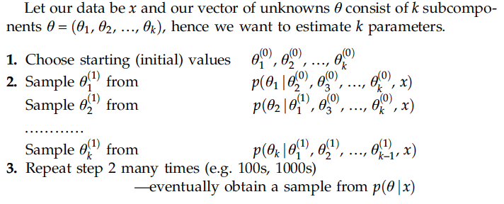
One iteration includes as many random draws as there are parameters in the model; in other words, the chain for each parameter is updated by using the last value sampled for each of the other parameters, which is referred to as full conditional sampling.
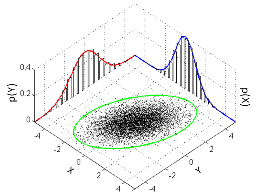
Figure 4.5: Visualizing parameter sampling
Although the nuts and bolts of MCMC can get very detailed and may go beyond the operational knowledge you need to run models, there are some practical issues that you will need to be comfortable handling, including initial values, burn-in, convergence, thinning,
4.3.4 Burn-in
- Chains start with an initial value that you specify or randomize
- Initial value may not be close to true value
- This is OK, but need time for chain to find correct parameter space
- If you know your high probability region, then you may have burned in already
- Visual Assessment can confirm burn-in
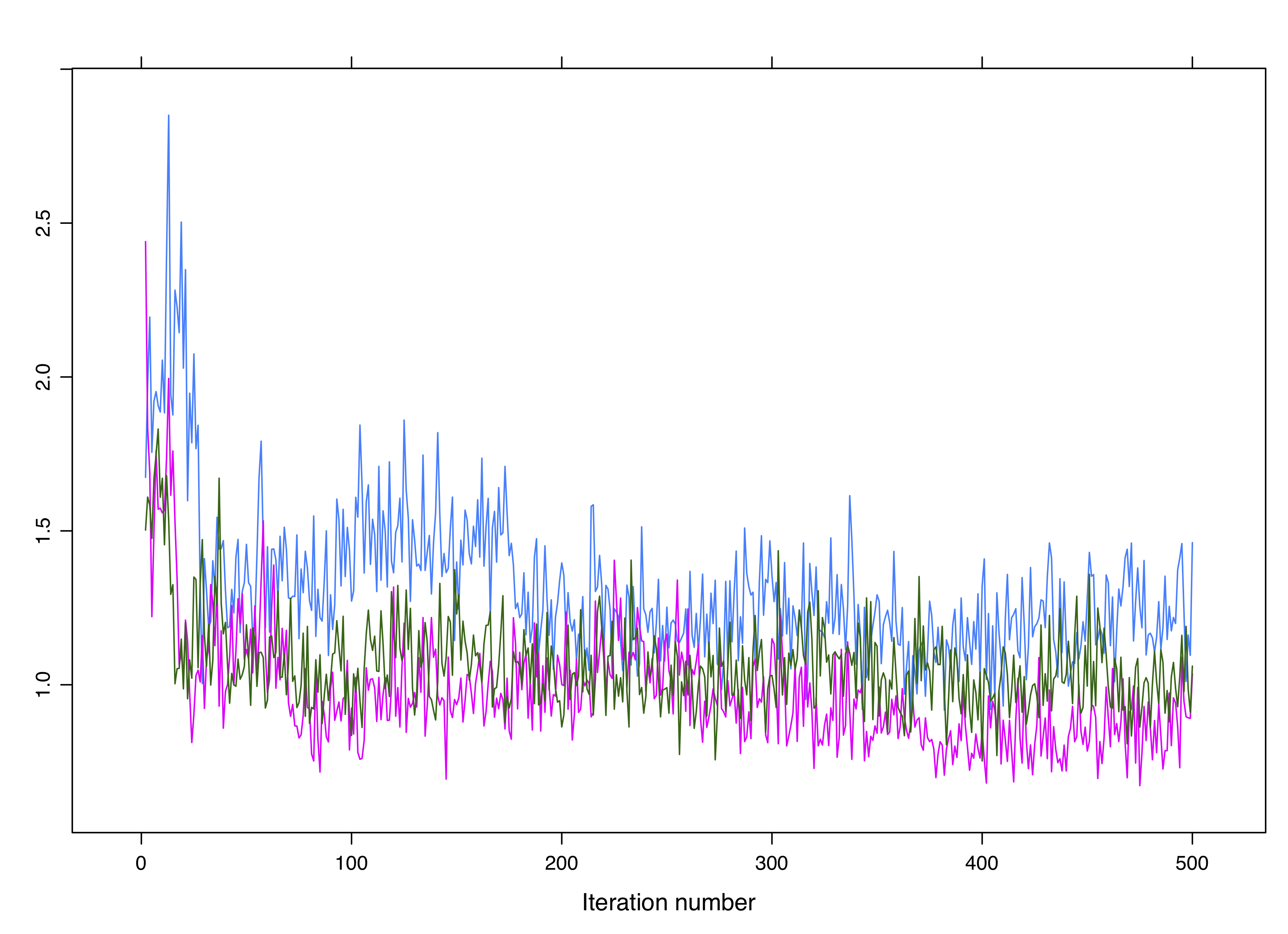
Figure 4.6: Burn-in is the initial MCMC sampling that may take place outside of the highest probability region for a parameter.
4.3.5 Convergence
- We run multiple independent chains for stronger evidence of correct parameter space
- I When chains converge on the same space, that is strong evidence for convergence
- But how do we know or measure convergence?
- Averages of the functions may converge (chains don’t technically converge)
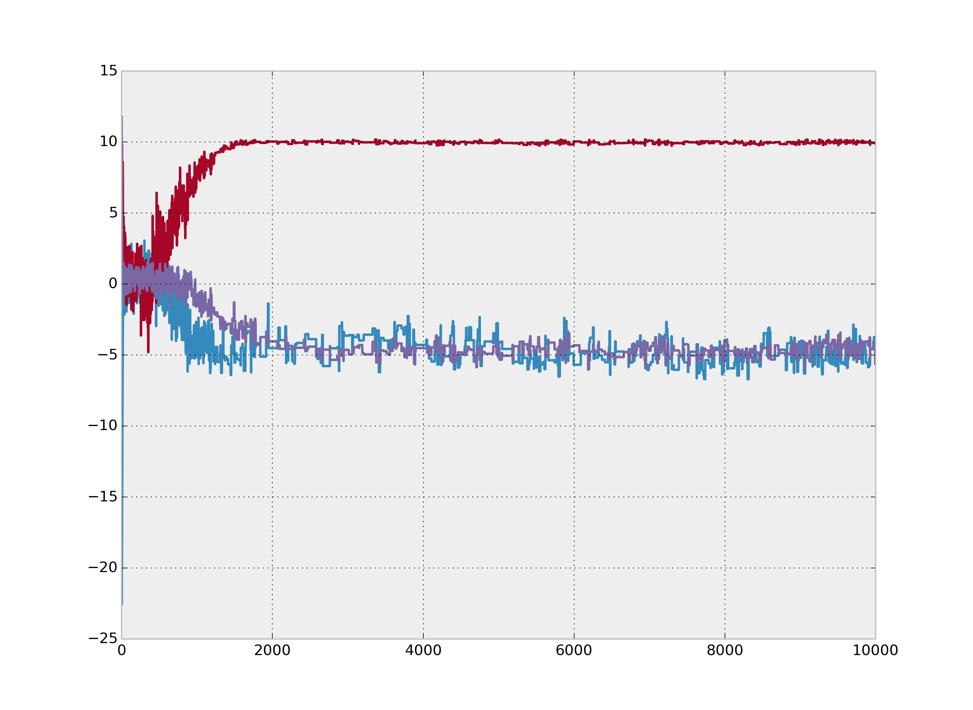
Figure 4.7: Clean non-convergence for 3 chains.
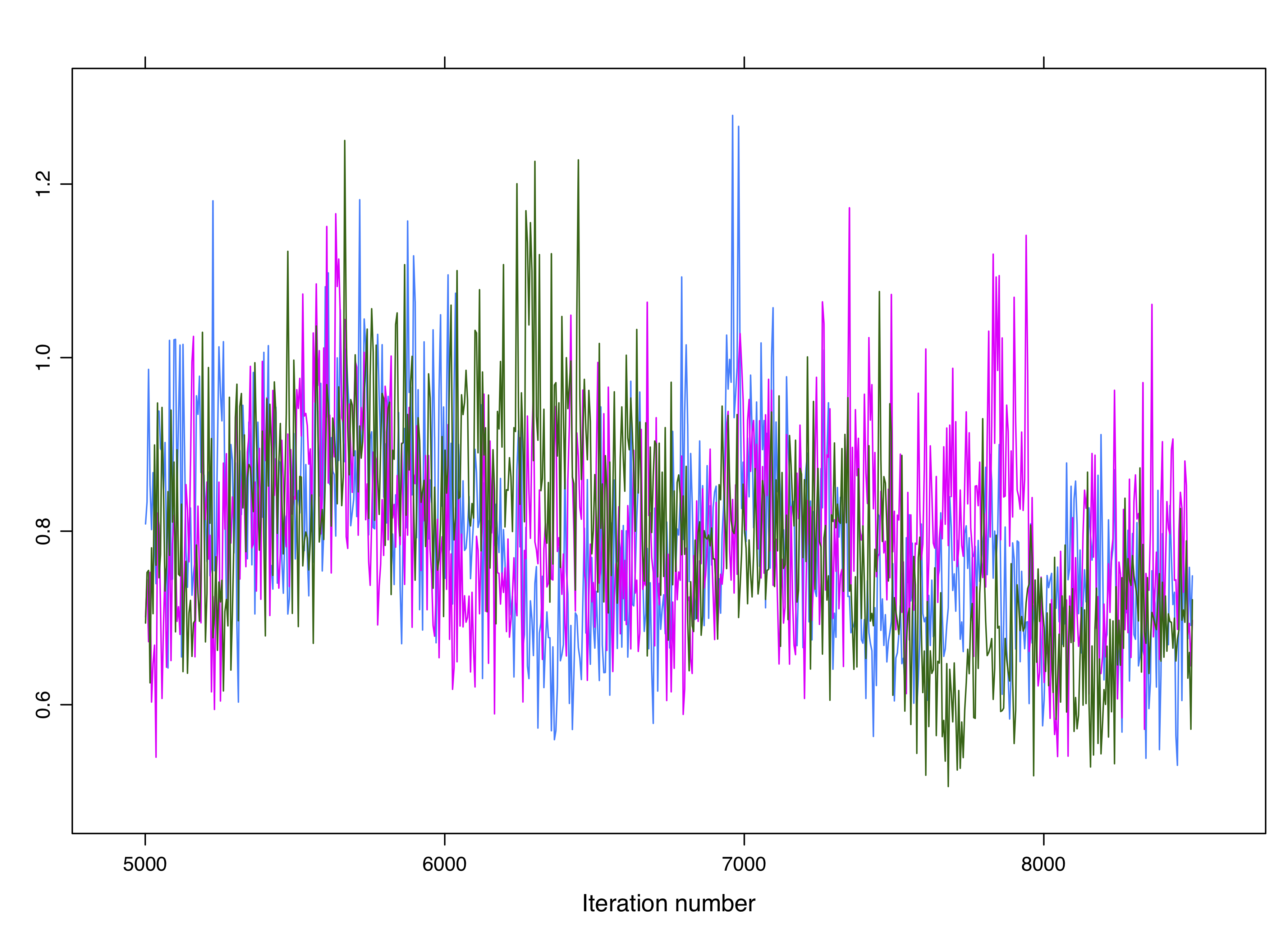
Figure 4.8: Non-convergence is not always obvious. These chains are not converging despite overlapping.
Convergence Diagnostics
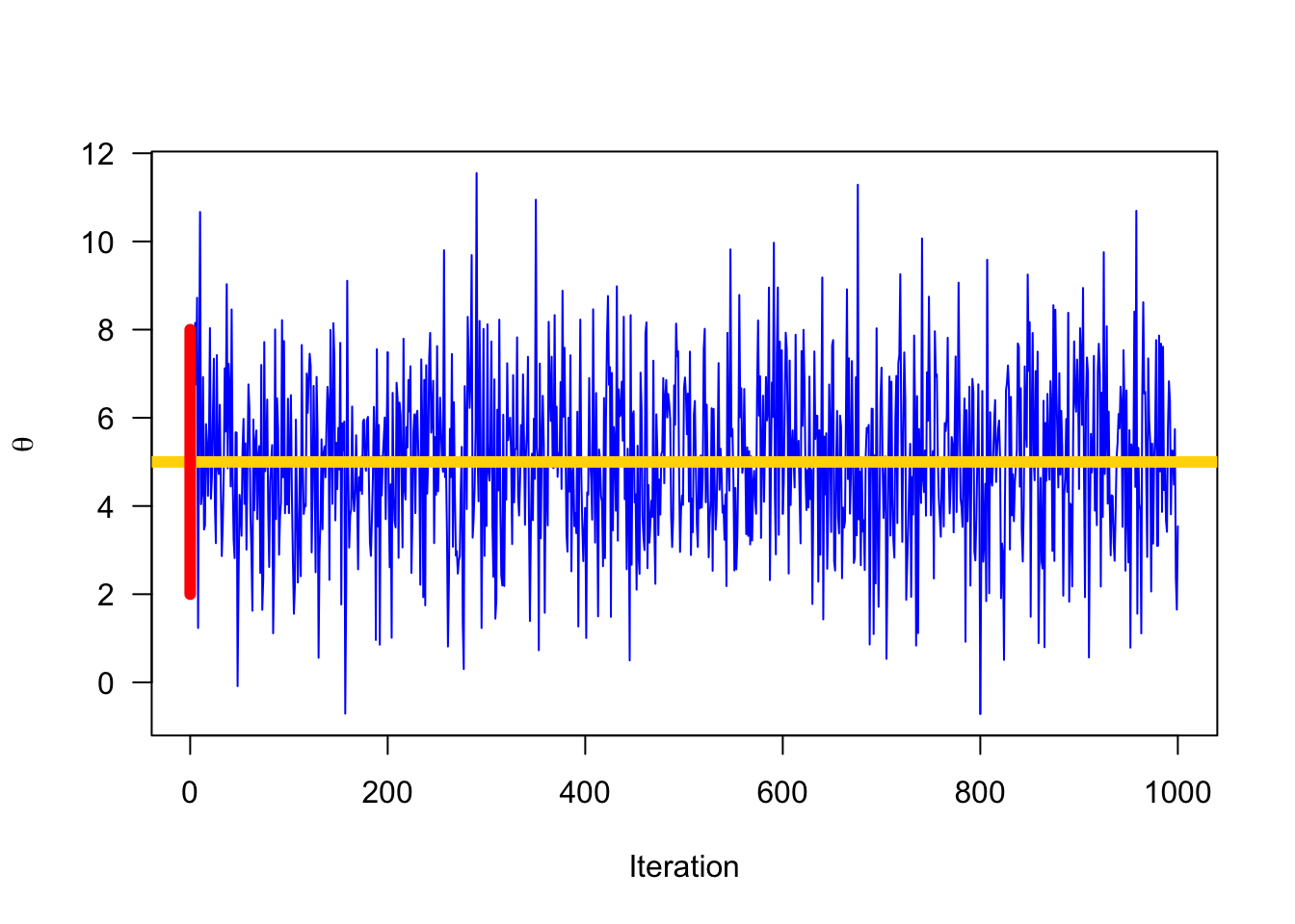
- Visual convergence of iterations (“hairy caterpillar” or the “grass”)
- Visual convergence of histograms
- Brooks-Gelman-Rubin Statistic, \(\hat{R}\)
- Others
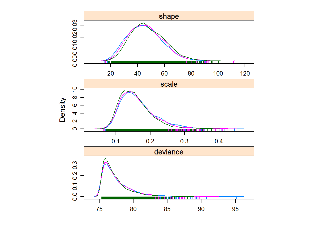
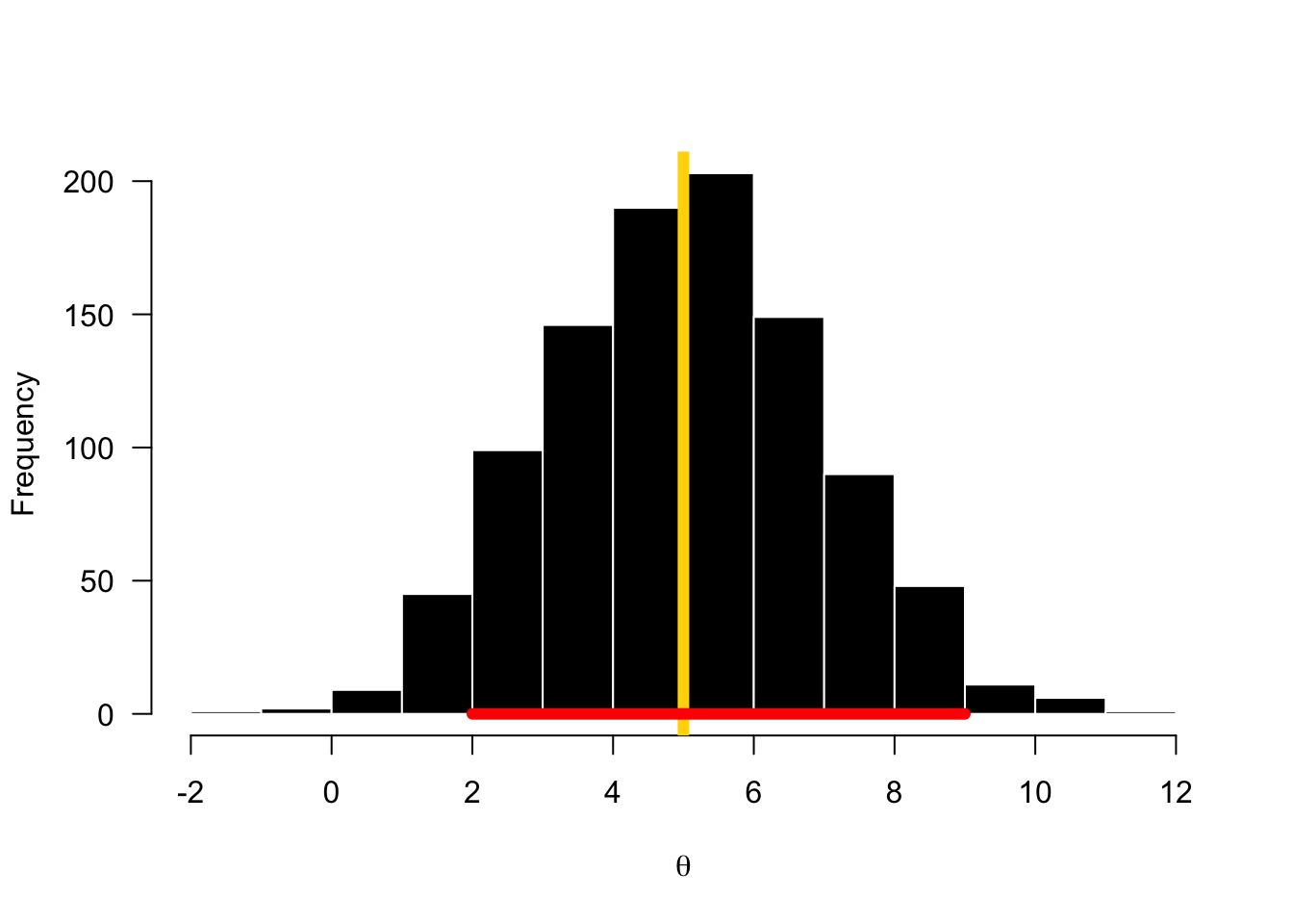
Figure 4.9: Histograms and density plots are a good way to visualize convergence.
4.3.6 Thinning
MCMC chains are autocorrelated, so \(\hat{\theta_t} \sim f(\hat{\theta}_{t-1})\). It s common practice to thin by 2, 3 or 4 to reduce autocorrelation. However, there are also arguements against thinning.
4.3.7 MCMC Summary
There is some artistry in MCMC, or at least some decision that need to be made by the modeler. Your final number of samples in your posterior is often much less than your total iterations, because in handling the MCMC iterations you will need to eliminate some samples (e.g., burn-in and thinning). Many MCMC adjustments you make will not result in major changes, and this is typically a good thing because it means you are in the parameter space you need to be in. Other times, you will have a model issue and some MCMC adjustment will make a (good) difference. Because computation is cheap—especially for simple models—it is common to over-do the iterations a little. This is OK.
Here is a nice overview video about MCMC. https://www.youtube.com/watch?v=OTO1DygELpY
And here is a great simulator to play with to evaluate how changes in MCMC settings play out visually. https://chi-feng.github.io/mcmc-demo/app.html