Chapter 3 Fundamentals of Bayesian Inference
3.1 Models vs. Estimation
Need text on actual difference between models and estimation.
Observations are a function of observable and unobservable influences. We can think about the observable influences as data and the unobservable influences as parameters. But even with this breakdown of influences, most systems are too complex to look at and understand. Consider the effects of time, space, unknown factors, interactions of factors, and other things that obscure relationships. One approach is to start with a simple model that we might know is wrong (i.e., incomplete), but which can be known and understood. Any model is necessarily a formal simplification of a more complex system and no models are perfect, despite the fact they can still be useful. By starting with a simple model we can add complexity as we understand it and hypothesize the mechanisms, rather than trying to start with with a complex model that might be hard to understand and work with.
A lot of good things have been said about models, including:
“All models are wrong, but some are useful” -George Box
“There has never been a straight line nor a Normal distribution in history, and yet, using assumptions of linearity and normality allows, to a good approximation, to understand and predict a huge number of observations.” -W.J. Youden
“Nothing is gained if you replace a world that you don’t understand with a model that you don’t understand.” -John Maynard Smith
3.1.1 Model Building
Most model selection procedures attempt balance between model generalizability and specificity, and in putting a model together this balance is also importnat. Consider whether you seek prediction or understanding; although they may overlap they do have differences. Model (system) understanding may not predict well, but can help to explain drivers of a system. On the other hand model prediction may not explain well, but the value is in performance. Often, prediction and understanding are not exclusive and thought needs to be given to the balance of both in a model. Let’s consider prediction and understanding a little more.
Explanation (understanding)
- Emphasis on understanding a system
- Often simpler models (but not always!)
- Strong focus on parameters, which represent your hypothesis of the system
- Think: Causes of effects
Prediction
- Focus on fitting \(y\)
- Often result more complex models (but not always!)
- Think: Effects of causes
3.1.2 Case Study: Explanation vs Prediction
Reproductive biological work on Southern Flounder (Paralichthys lethostigma) was conducted to determe predictors associated with oocyte development and expected spawning. Becuase the species, like many other fish species, are not observed on the spawning grounds all information about maturity has to be collected prior to fully-developed, spawning capable individuals are available. A wide range of predictors were quantified to examine their correlation to histological samples of ovarian tissue. In addition to identifying reliable predictors, value was placed on simplicity—the fewer predictors needed, the more useful the model would be.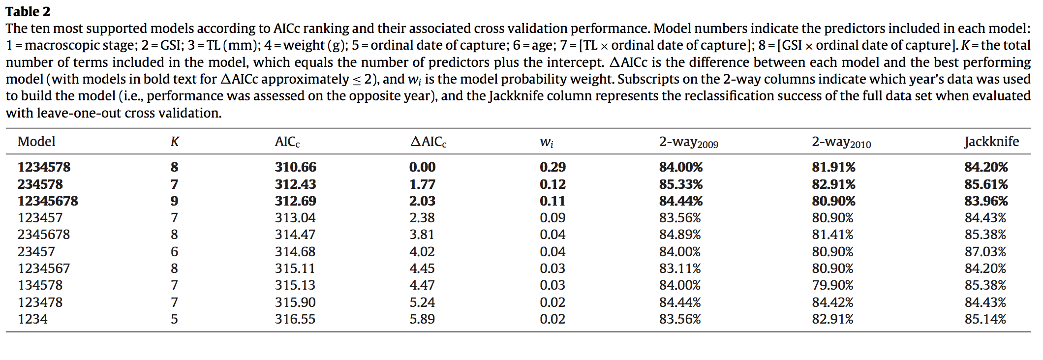
Figure 3.1: Table of best-fitting models as determined by AIC (Midway et al. 2013).
AIC was able to determine a best-fitting model; however, there were several competing models all of which tended to have a large number of predictors.
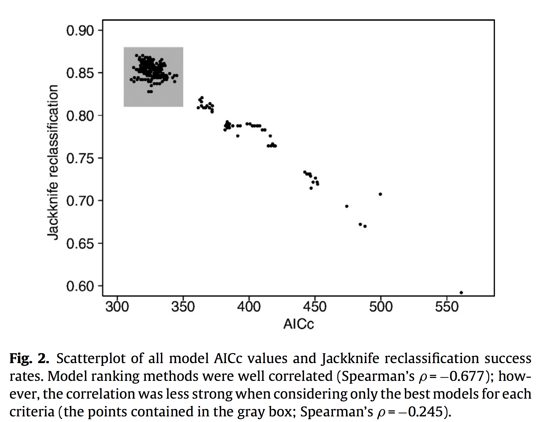
Upon closer evaluation, it appeared that a large number of models all performed relatively well, when compared with each other. This cloud of model points warranted further investigation.
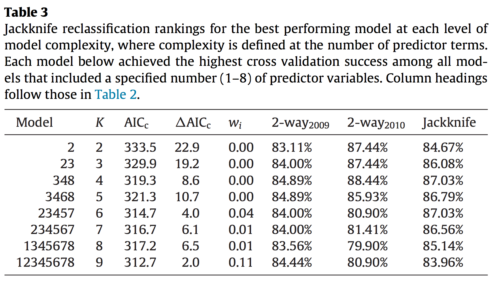
When evaluating model perfomance based on cross-validation, a large number of simpler models were found to be effective. These results highlight that for this particular dataset system understanding was optimized by AIC, while system prediction was optimzed by cross-validation.
3.1.3 Models vs Estimation
Consider a simple linear regression model: \(y_i = \alpha + \beta \times x_i + \epsilon_i\). How might we come up with estimates of the model parameters, namely \(\alpha\), and \(\beta\)? To do this, we need and estimation routine, and there is more than one to choose from. It’s important to know that the estimatation routine we select will have different operating assumptions, different underlying machinery, and may produce different results (estimates). That being said, for simple models and clear data, different estimation routines may result in very similar outcomes. Regardless, it remains very important to remember that both models and estimation are independent components of statistics. We might all agree on a model, but not the estimation (or the opposite). The linkage between models and estimation is often the parameters; parameters are what define a model, and parameters can be estimated by different methods.
“…there is no `Bayesian so-and-so model’.” Kéry and Schaub (2011)
3.1.4 What is a parameter?
Parameters are system descriptors. Think of a parameter as something that underlies and influences a population, whereas a statistic does the same for a sample. For example, a population growth rate parameter, \(lambda\), may describe the rate of change in the size of a population, whereas some difference statistic, \(N_d\) may describe the difference in the size of the population between some time interval. In addition to making sure we know the parameters—and their configuration—that serve as hypotheses for systems and processes, the interpretation of parameters is also at the foundation for different statistical estimation procedure and philosphies.
3.2 Bayesian Basics
Figure 3.2: An attempt at humor while illustrating different statistical philosophies.
3.2.1 Why learn Bayesian estimation?
“Our answer is that the Bayesian approach is attractive because it is useful. Its usefulness derives in large measure from its simplicity. Its simplicity allows the investigation of far more complex models than can be handled by the tools in the classical toolbox.” Link and Barker (2009)
In order to understand and command complexity, you need to revisit simplicity—and when you go back to basics, you gain deeper understanding." Midway
Figure 3.3: The Reverend Thomas Bayes
Thomas Bayes was a Presbyterian Minister who is thought to have been born in 1701 and died 1761. He posthumously published An Essay towards solving a Problem in the Doctrine of Chances in 1763, in which he introduced his approach to probability. Bayesian approach were never really practiced in Bayes’ lifetime—not only was his work no published until after he died, but his work then was not developed and popularized until Pierre-Simon Laplace (1749–1827) did so in the early 19th century. (Fun fact according to Wikipedia: His [Laplace] brain was removed by his physician, François Magendie, and kept for many years, eventually being displayed in a roving anatomical museum in Britain. It was reportedly smaller than the average brain.)
Bayes’ rule, in his words:
Given the number of times in which an unknown event has happened and failed: Required the chance that the probability of its happening in a single trial lies somewhere between any two degrees of probability that can be named.
- “unknown event” = e.g., Bernoulli trial
- “probability of its happening in a single trial” = \(p\)
- We may know ahead of time, or not
Consider an example where 10 chicks hatch and 4 survive. Bayes attempts to draw a conclusion, such as “The probability that \(p\) (survival) is between 0.23 and 0.59 is 0.80.” The two degrees of probability are an interval; \(Pr(a \leq p \leq b)\). The overall idea is similar to a confidence interval in trying to account for and reduce uncertainty—but confidence intervals are not probabilistic, so they are are not the same.
A key distinction between Bayesian and Frequentists is how uncertainty regarding parameter \(\theta\) is treated. Frequentists views parameters as fixed and probability is the long run probability of events in hypothetical datasets. The result is that probability statements are made about the data—not the parameters! A Frequentist could never state: “I am 95% certain that this population is declining.” (Note: in order to learn about Bayesian approaches from a practical standpoint, we will often consider it against the Frequentists approach for comparison.)
But for a Bayesian, probability is the belief that a parameter takes a specific value. “Probability is the sole measure of uncertainty about all unknown quantities: parameters, unobservables, missing or mis-measured values, future or unobserved predictions” (Kéry and Schaub 2011). When everything is a probability, we can use mathematical laws of probability. One way to get started is to think of parameters as random variables (but technically they are not.)
3.2.2 Bayesian vs. Frequentist Comparison
- Both start with data distribution (DGF)
- Data, \(y\), is a function of parameter(s), \(\theta\)
- Example: \(p(y|\theta) \sim Pois(\theta)\) which is often abbreviated to \(y|\theta \sim Pois(\theta)\) or \(y \sim Pois(\theta)\)
- Frequentist then uses likelihood function to interpret distribution of observed data as a function of unknown parameters, \(L(\theta |y)\). But, likelihoods do not integrate to 1, and are therefore not probabilistic
- Frequentist estimate a single point, the maximum likelihood estimate (MLE), which represents the parameter value that maximizes the chance of getting the observed data
- see Kéry and Schaub (2011) for extended example of MLE
3.2.3 Bayesians use Bayes’ Rule for inference
\[P(A|B)=\frac{P(B|A)\times P(A)}{P(B)}\]
Bayes’ Rule is a mathemetical expression of the simple relationship between conditional and marginal probabilities.
Example of Bayes’ Rule Bird watching (B) or watching football (F), depending on good weather (g) or bad weather (b) on given day.
We know:
- \(g + B = 0.5\) (joint)
- \(g = 0.6\) (marginal)
- \(B = 0.7\) (marginal)
If you are watching football, what is the best guess as to the weather?
| Good Weather (g) | Bad Weather (b) | ||
|---|---|---|---|
| Bird watching (B) | 0.5 | 0.2 | 0.7 |
| Watch Football (F) | 0.1 | 0.2 | 0.3 |
| 0.6 | 0.4 | 1.0 |
Rephrased, we are asking \(p(b|F)\)
We know:
- \(p(b, F) = 0.2\)
- \(p(F) = 0.3\)
- \(p(b|F) =\) \(\frac{p(b,F)}{p(F)} =\) \(\frac{0.2}{0.3} =\) 0.66
The probability of bad weather is 0.4, but knowing football is more likely with bad weather, football increased our guess to 0.66.
3.2.4 Breaking down Bayes’ Rule
\[P(\theta|y)=\frac{P(y|\theta)\times P(\theta)}{P(y)}\]
where
- \(P(\theta|y)\) = posterior distribution
- \(P(y|\theta)\) = Likelihood function
- \(P(\theta)\) = Prior distribution
- \(P(y)\) = Normalizing constant
Another way to think about Bayes’ Rule \[P(\theta|y) \propto P(y|\theta)\times P(\theta)\] Combine the information about parameters contained in the data \(y\), quantified in the likelihood function, with what is known or assumed about the parameter before the data are collected and analyzed, the prior distribution.
3.3 Bayesian and Frequentist Comparison
3.3.1 Example with Data
Consider this simple dataset of two groups each with 8 measurements.
y <- c(-0.5, 0.1, 1.2, 1.2, 1.2, 1.85, 2.45, 3.0, -1.8, -1.8, -0.4, 0, 0, 0.5, 1.2, 1.8)
g <- c(rep('g1', 8), rep('g2', 8))
We might want to consider a \(t\)-test to compare the groups (means). In this case, we are estimating 5 parameters from 16 data points.
##
##  Welch Two Sample t-test
##
## data:  y by g
## t = 2.2582, df = 13.828, p-value = 0.04064
## alternative hypothesis: true difference in means is not equal to 0
## 95 percent confidence interval:
##  0.06751506 2.68248494
## sample estimates:
## mean in group g1 mean in group g2
##           1.3125          -0.0625
Our t-test results in a p-value of 0.0406, which is less than the traditional cutoff of 0.05 and allowing us to conclude that the group means are significantly different. At this point in our study, we would write up our model results and likely conclude the analysis. The frequentist t-test is simple, but limited.
Let’s try a Bayesian t-test.
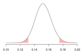
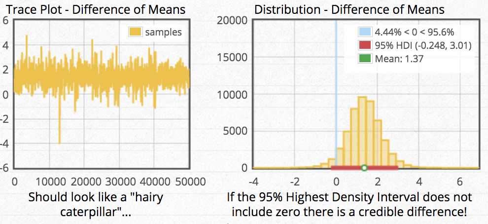 Here we see a posterior distribution of our results. The mean difference between groups was estimated to be 1.37, and the 95% credible interval around that difference is reported as -0.248 to 3.01. A credible interval represents the percentage (95% in this case) of symmetric area under the distribution that represents the uncertainty in our point estimate. The percentage can also be used to interpret the chance that the interval has captured the true parameter. So in this example, we can say that we are 95% certain that the true difference in means lies between -0.248 and 3.01, with our best guess being 1.37. Another thing we can use credible intervals for is “significance” interpretation. If a credible interval overlaps 0, it can be interpreted that 0 is within the range of possible estimates and therefore there is no significant interpretation. (If 0 were to be outside our 59% CI, we would have evidence that 0 is not a very likely estimate and therefore the group means are “statistically significant.”) It’s worth noting that the concept of statistical significance may be alive and well in Bayesian esimation; however, you need to define how the term is used because there is no a priori significance level as there is in frequentist routines.
Consider also that the frequentist t-test found a significant difference and the Bayesian t-test did not find a difference. In reality, with simple (and even more complex) datasets, both types of estimation will often arrive at the same answer. This example was generated to show that there is the possibility to reach different significance conclusions using the same data. Perhaps what is more important in this example is to ask yourself if two types of estimation reach different conclusions about the data, which are you more likely to trust—the procedure that provides little information and spits out a yes or no, or the procedure that is full tractable and provides results and estimation for all parts of the model?
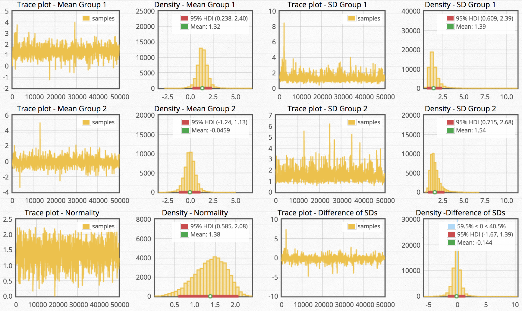 But wait—there’s more! Because Bayesian estimation assumes underlying distributions for everything, we get richer results. All estimated parameters have their own posterior distributions, even the group-specific standard deviations.
Despite the benefits illustrated in this example, it’s important to know that the Bayesian approach is not inherently the correct way to appraoch estimation. In fact, we cannot know which method is correct. All we can know is that we are presented with a choice as to which method provides richer information from which we can base a decision.
3.3.2 More differences
Frequentists: \(p(data|\theta)\)
- Data are repeatable, random variables
- Inference from (long-run) frequency of data
- Parameters do not change (the world is fixed and unknowable)
- All experiments are (statistically) independent
- Results driven by point-estimates
- Null Hypothesis emphasis; accept or reject
Bayesians: \(p(\theta |data)\)
- The data are fixed (data is what we know)
- Parameters are random variables to estimate
- Degree-of-belief interpretation from probability
- We can update our beliefs; analyses need not be independent
- Driven by distributions and uncertainty
3.3.3 Put another way
Frequentists asks: The world is fixed and unchanging; therefore, given a certain parameter value, how likely am I to observe data that supports that parameter value?
Bayesian asks: The only thing I can know about the changing world is what I can observe; therefore, based on my data, what are the most likely parameter values I could infer?
Given the strengths and weaknesses for both types of estimation, why did the Frequentist approach dominate for so long, even to the present? The best explanation includes several reasons. Frequentist routines are computationally simple compared to Bayesian appraoches, which has permitted them to be formalized into point-and-click routines that are available to armchair statisticians. Additionally, the create and popularization of ANOVA ran parallel to the rise in popularity of Frequentist appraoches, and ANOVA provided an excellent model for many data sets. Finally, although the limitations and issues with p-values are well-publicized, there has been historic appeal for statistical complexity being reduced to a significant or non-significant outcome.
3.3.4 Uncertainty: Confidence Interval vs Credible Interval
Consider the point estimate of 5:12 and the associated uncertainty of 4:12–6:12
Frequentist interpretation: Based on repeated sampling, 95% of intervals contain the true, unknowable parameter. Therefore, there is a 95% chance that 4.12–6.12 contains the true parameter we are interested in.
Bayesian interpretation: Based on the data, we are 95% certain that the interval 4.12–6.12 contains the parameter value, with the most likely value being 5.12 (the mean/mode of the distribution).
These are different interpretations!
3.3.5 Bayesian Pros and Cons
Pros
- Can accomodate small samples sizes
- Uncertainty accounted for easily
- Degree-of-belief interpretation
- Very flexible with respect to model design
- Modern computers make computation possible
Cons
- Still need to code (but also a pro?)
- Still computationally intensive in some applications
Other Practical Advantages of Bayesian Estimation
- Easy to use different distributions (e.g., t-test with t-distribution)
- Free examination and comparisons
- Comparing standard deviations
- Comparing factor levels
- The data don’t change, why should the p-value?
- Uncertainty for ALL parameters and derived quantities
- Credible intervals make more sense than confidence intervals
- Probabilistic statements about parameters and inference
- With diffuse priors, approximate MLE (no estimation risk)
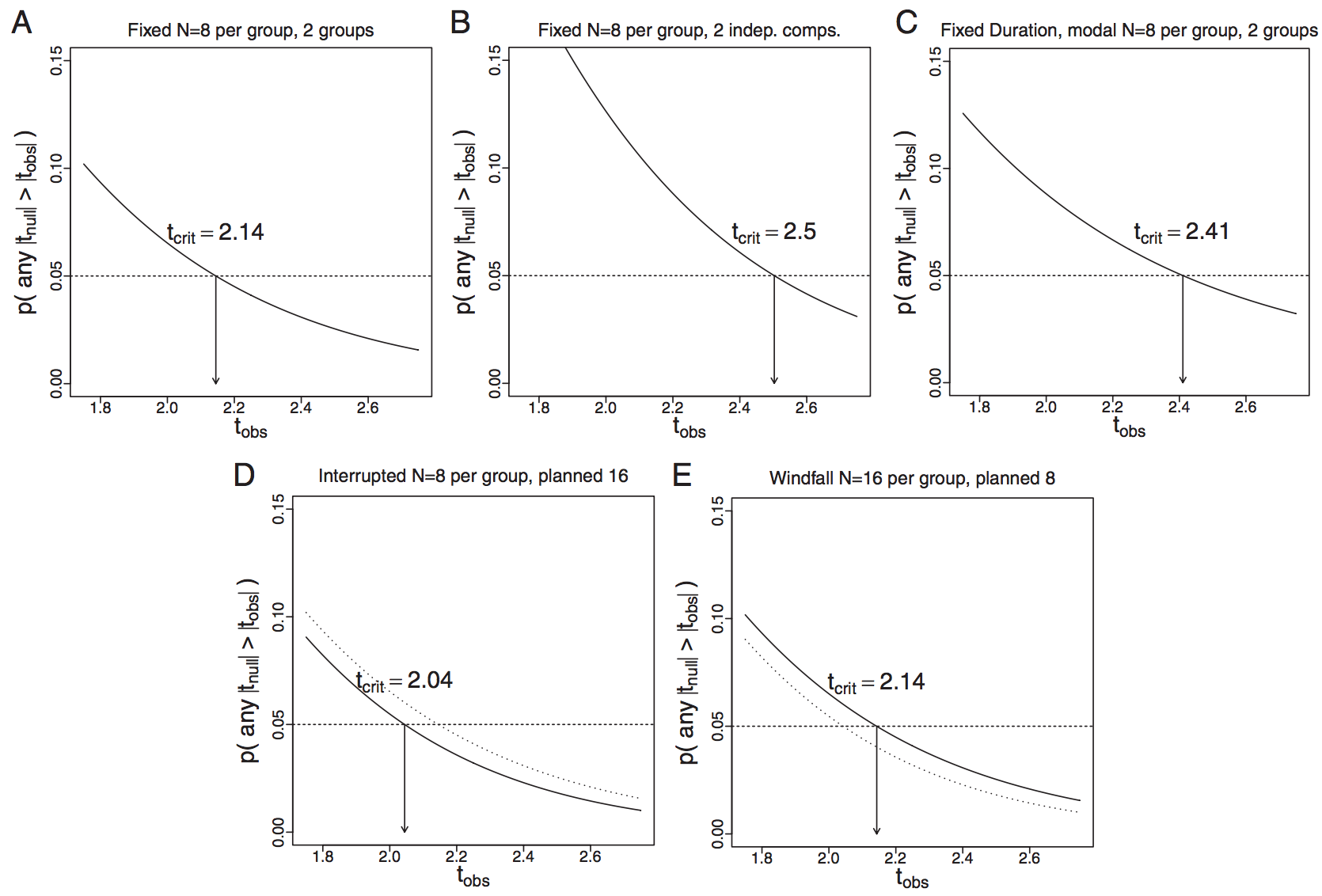
- Test statistics and model outcome NOT dependent on sampling intentions
- Frequentists experiments need a priori sample size (do you do this?)
- Test statistics vary, which means p-values vary, which means decisions change
- The data don’t change, why should the p-value?
References
Kéry, Marc, and Michael Schaub. 2011. Bayesian Population Analysis Using Winbugs: A Hierarchical Perspective. Academic Press.
Link, William A, and Richard J Barker. 2009. Bayesian Inference: With Ecological Applications. Academic Press.