Chapter 2 The Model Matrix and Random Effects
2.1 Linear Models
Let’s start with reviewing some linear modeling terminology.
- units–observations; i , data points
- x variable–predictor(s); independent variables
- y variable–outcome, response; dependent variable
- inputs–model terms; \(\neq\) predictors; inputs \(\geq\) predictors
- random variables–outcomes that include chance; often described with probability distribution
- multiple regression–regression of > 1 predictor; not multivariate regression (MANOVA, PCA, etc.)
The general components of a linear model can be thought of as any of the following:
response \(=\) deterministic \(+\) stochastic
outcome \(=\) linear predictor \(+\) error
result \(=\) systematic \(+\) chance
- The stochastic component makes these statistical models
- Explanatory variables whose effects add together
- Not necessarily a straight line!
2.1.1 Stochastic Component
- Nature is stochastic; nature adds error, variability, chance
- Always a reason, we might just not know it
- Might not be important and including it risks over-parameterization
- Combined effect of unobserved factors captured in probability distribution
- Often (default) is Normal distribution, but others common
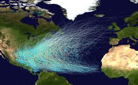
Figure 2.1: Although hurricanes are not statistical models, they are a good example of understanding something that cannot perfectly be modeled, and therefore has some stochasticity inherent to it.
In a linear model, we need to identify a distribution that we assume is the data generating distribution underyling the process we are attempting to model. Not only is this distrubtion important in describing what we are modeling, but it is also critically important because it will accomodate the errors that arise when we model the data. So how do we know which distribution we need for a given model?
- We can know possible distributions
- We can know how data were sampled
- We can know characteristics of the data
- We can run model, evaluate, and try another distribution
- Correct distribution is not always Y/N answer
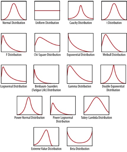
Figure 2.2: Examples of different statistical distributions as seen by their characterstic shape.
2.1.2 Distributions
Although many distributions are available, we will review three.
- Normal distribution: continuous, \(-\infty\) to \(\infty\)
- Binomial distribution: discrete, integers, 0 to 1
- Poisson distribution: discrete, integers, 0 to \(\infty\)
The Normal distribution
The normal distribution is the model common distribution in linear modeling and possible the most common in nature. In a normal distribution, measurements effected by large number of additive effects (CLT). When effects are multiplicative, the result is a log-normal distribution. There are 2 parameters that govern the normal distribution: \(\mu\) = mean and \(\sigma^2\) = standard deviation.
A normal distribution can be easily simulated in R.
##  [1] -0.5954732  1.1289288  0.3290828 -0.8824579 -0.2629276  0.2449900
##  [7]  2.0645695  0.7203280  0.4977901  0.5770971
The Binomial distribution
The binomial distribution always concerns the number of successes (i.e., a specific outcome) out of a total number of trials. A single trial is a special case of the binomial, and is called a Bernoulli trial. The flip of a coin once is the classic Bernoulli trial. A binomial distribution might be thought of as the sum of some number of Bernoulli trials. A binomial distibution has 2 parameters: \(p\) = success probability and \(N\) = sample size (although \(N\)=1 in a Bernoulli trial, which means a Bernoulli trial can be thought of as a 1-parameter distribution). \(N\) is the upper limit, which differentiates from a binomial distribution from a Poisson distribution. The binomial distribution mean is a derived quantity, where \(\mu = N \times p\). the variance \(= N \times p \times (1 - p)\); therefore, the variance is function of mean.
A binomial distribution can be simulated in R.
## [1] 0 1 2 1 0 1 2 2 3 1The Poisson distribution
The Poisson distribution is the classic distribution for (integer) counts; e.g., things in a plot, things that pass a point, etc.) The Poisson distribution can approximate to Binomial when \(N\) is large and \(p\) is small, and it can approximate to the normal distribution when when \(\lambda\) is large. The Poisson distribution has 1 parameter: \(\lambda\) = mean = variance. This distribution can be modified for zero-inflated data (ZIP) and other distributional anomolies.
A Poisson distribution can be easily simulated in R.
## [1] 2 1 8 6 2 4 4 2 2 22.1.3 Linear Component
Recall that the linear contribution to our model includes the predictors (explanatory variables) with additive effects. Although this is a linear model, it need not be thought of literally as a straight line. The linear component can accomodate both continuous and categorical data. Conceptually,
linear predictor \(=\) design matrix \(+\) parameterization
R takes care of both the design matrix and the parameterization, but this is not always true in JAGS, so it is worth a review.
Marc Kery has succinctly summarized the design matrix:
“For each element of the response vector, the design matrix \(n\) index indicates which effect is present for categorical (discrete) explanatory variables and what amount of an effect is present in the case of continuous explanatory variables.” (Kéry 2010)
In other words the design matrix is a matrix that tells the model if and where an effect is present, and how much. The number of columns in the matrix are equal to the number of fitted parameters. Ultimatly, the design matrix is multiplied with the parameter vector to produce the linear predictor. Let’s use the simulated data in Chapter 6 of Marc Kery’s book as an example (Kéry 2010).
| mass | pop | region | hab | svl |
|---|---|---|---|---|
| 6 | 1 | 1 | 1 | 40 |
| 8 | 1 | 1 | 2 | 45 |
| 5 | 2 | 1 | 3 | 39 |
| 7 | 2 | 1 | 1 | 50 |
| 9 | 3 | 2 | 2 | 52 |
| 11 | 3 | 2 | 3 | 57 |
If you would like to code this dataset into R and play along, use the code below.
mass <- c(6,8,5,7,9,11)
pop <- c(1,1,2,2,3,3)
region <- c(1,1,1,1,2,2)
hab <- c(1,2,3,1,2,3)
svl <- c(40,45,39,50,52,57)
If we think about a model of the mean, it might look like this:
\[mass_i=\mu + \epsilon_i\]
This model has a covariate of one for every observation, because every observation has a mass. This model is also sometimes referred to as an intercept only model. The model describes individual snake mass as a (global) mean plus individual variation (deviation or “error”).
Increasing model complexity, we might hypothesize that snake mass is predicted by region. Because region is a categorial variable (although it is input as numeric, we don’t assume any ordination or relationship of the region numbers), the model we are interested in is a \(t\)-test. A \(t\)-test is just a specific case of a linear model. To represent the \(t\)-test, we can write the model equation as:
\[mass_i = \alpha + \beta \times region_i + \epsilon_i\]
This model is considering snake mass to be made up of these components: the mean snake mass, the region effect, and the residual error. Now is also a good time to start thinking about the residuals, which we assume are normally distributed with a mean of 0 and expresed as
\[\epsilon_i \sim N(0,\sigma^2)\]
Let’s pause for a moment on the \(t\)-test and think about how we write models. You are familiar with the notation that I have thus used, where the model and residual error are expressed as two separate equations. What if we were to combine them into one equation? How would that look?
\[mass_i \sim N(\alpha + \beta \times region_i, \sigma^2)\]
This notation may take a little while to get used to, but it should make sense. This expression is basically saying that snake mass is thought to be normally distributed with a mean that is the function of the mean mass plus region effect, and with some residual error. Expressing models with distributional notation may seen odd at first, but it may help you better understand how distributions are built into the processes we are modeling, and what part of the process belongs to which part of the distribution. We will stick with this notation (not exclusively) for much of this course.
Back to the model matrix—how might we visualize the model matrix in R?
##   (Intercept) region
## 1           1      1
## 2           1      1
## 3           1      1
## 4           1      1
## 5           1      2
## 6           1      2
## attr(,"assign")
## [1] 0 1
But we said earlier the regions were not inherent quantities and just categories or indicator variables. Above, R is taking the region variable as numeric because it does not know any better. Let’s tell R that region is a factor.
##   (Intercept) as.factor(region)2
## 1           1                  0
## 2           1                  0
## 3           1                  0
## 4           1                  0
## 5           1                  1
## 6           1                  1
## attr(,"assign")
## [1] 0 1
## attr(,"contrasts")
## attr(,"contrasts")$`as.factor(region)`
## [1] "contr.treatment"
The model matrix yields a system of equations. And for the matrix above, the system of equations we would have can be expressed 2 ways. The first way shows the equation for each observation.
\[6=\alpha \times 1 + \beta \times 0 + \epsilon_1\] \[8=\alpha \times 1 + \beta \times 0 + \epsilon_2\] \[5=\alpha \times 1 + \beta \times 0 + \epsilon_3\] \[7=\alpha \times 1 + \beta \times 0 + \epsilon_4\] \[9=\alpha \times 1 + \beta \times 1 + \epsilon_5\] \[11=\alpha \times 1 + \beta \times 1 + \epsilon_6\]
The second way adopts matrix (vector) notation to economize the system.
\[\left(\begin{array} {c} 6\\ 8\\ 5\\ 7\\ 9\\ 11 \end{array}\right) = \left(\begin{array} {cc} 1 \hspace{3mm}0\\ 1 \hspace{3mm}0\\ 1 \hspace{3mm}0\\ 1 \hspace{3mm}0\\ 1 \hspace{3mm}1\\ 1 \hspace{3mm}1\\ \end{array}\right) \times \left(\begin{array} {c} \alpha \\ \beta \end{array}\right) + \left(\begin{array} {c} \epsilon_1\\ \epsilon_2\\ \epsilon_3\\ \epsilon_4\\ \epsilon_5\\ \epsilon_6 \end{array}\right) \]
In both cases the design matrix and parameter vector are combined. And using least-squares estimation to estimate the parameters will result in the best fits for \(\alpha\) and \(\beta\).
2.1.4 Parameterization
Although parameters are inherent to specific models, there are cases in the linear model where parameters can be represented in different ways in the design matrix, and these different representations will have different interpretations. Typically, we refer to either a means or effects parameterization. These two parameterizations really only come into play when you have a categorical variable—the representation of continuous variables in the model matrix includes the quantity or magnitude of that variable (and defaults to an effects parameterization). A means parameterization may be present or needed when categorical variables are present. Let’s take the above \(t\)-test example with 2 regions. As we notated the model above, \(\alpha = \mu\) for region 1, and \(\beta\) represented the difference in expected mass in region 2 compared to region 1. In other words, \(\beta\) is an estimate of the effect of being in region 2. As you guessed, this is an effects parameterization because region 1 is considered a baseline or reference level, and other levels are compared to this reference, hence the coefficients represent their effect. Effects parameterization is the default in R (e.g., lm()).
In a means parameterization, \(\alpha\) has the same interpretation—the mean for the first group. However, in a means parameterization, all other coefficients represent the means of those groups, which is actually a simpler imterpretation than the effects parameterization. Going back to our \(t\)-test, in a means parameterization \(\beta\) would represent the mean mass for snakes in region 2. Thus, no addition or subtraction of effects is required in a means parameterization. Both the means and effects parameterization will yield the same estimates (with or without some simple math), but it is advised to know which parameterization you are using. Additionally, as you work in JAGS you may need to use one parameterization over another, and understanding how their work and are interpreted is critically important.
Let’s look at one more model using the snake data. A simple linear regression will fit one continuous covariate (\(x\)) as a predictor on \(y\). Let’s look at the model for the snout-vent length (svl) as the predictor on mass.
\[mass_i = \alpha + \beta \times svl_i + \epsilon_i\]
The model matrix for this model (an effect parameterization) can be reported as such.
##   (Intercept) svl
## 1           1  40
## 2           1  45
## 3           1  39
## 4           1  50
## 5           1  52
## 6           1  57
## attr(,"assign")
## [1] 0 1
And we see that each snake has an intercept (mean) and an effect of svl.
These examples using the fake snake data were taken from Kery (2010), in which he provides more context and examples that you are encouraged to review.
2.2 Model Effects
To understand hierarchical models, we need to understand random effects, and to understand random effects, we need to understand variance.
- What is variance?
- How do we deal with variance?
- What can random effects do?
- How do I know if I need random effects?
- What is a hierarchical model? (later)
Variance was historically seen as noise or a distraction—it is the part of the data that the model does not capture well. At times it has been called a nuisance parameter. The traditional view was always that less variance was better. However:
“Twentieth-century science came to view the universe as statistical rather than as clockwork, and variation as signal rather than as noise…”(Leslie and Little 2003)
The good news is that there is (often) information in variance. Two problems, however, are that our models don’t always account for the information connected to variance, and that variance is often ubiquitous and can occur at numerous places within the model. For instance, variance can occur among observations and within observations, along with how we parameterize our models and how we take our measurements.
One way to deal with variance concerns how we treat the factors in our model. (Recall that a factor is a categorical predictor that has 2 or more levels.) Specifically, we can treat our factors as fixed or random, and the underlying difference lies in how the factor levels interact with each other.
2.2.1 Fixed Effects
Fixed effects are those model effects that are thought to be separate, independent, and otherwise not similar to each other.
- Likely more common—at least in use—than random effects, if only for the fact that they are a statistical default in most statistical softwares.
- Treat the factor levels as separate levels with no assumed relationship between them. _ For example, a fixed effect of sex might include two factor levels (male and female) that are assumed to have no relationship between them, other than that they are different types of sex.
- Without any relationship, we cannot infer what might exist or happen between levels, even when it might be obvious.
- Fixed effects are also homoscedastic, which means they assume a common variance.
- If you use fixed effects, you would likely need some type of post hoc means comparison (including adjustment) to compare the factor levels.
2.2.2 Random Effects
Random effects are those model effects that can be thought of as units from a distribution, almost like a random variable.
- Random effects are less commonly used, but perhaps more commonly encountered (than fixed effects).
- Each factor level can be thought of as a random variable from an underlying process or distribution.
- Estimation provides inference about specific levels, but also the population-level (and thus absent levels!)
- Exchangeability
- If \(n\) is large, factor level estimates are the same or similar to fixed effect estimates.
- If \(n\) is small, factor levels estimates draw information from the population-level information.
Comparing Effects Consider A is a fixed effect and B is a random effect, each with 5 levels. For A, inferences and estimates for the levels are applicable only to those 5 levels. We cannot assume to know what a 6th level would look like, or what a level between two levels might look like. Contrast that to B, where the 5 levels are assumed to represent an infinite (i.e., larger numbers) number of levels, and our inferences therefore extend beyond the data (i.e., we can use estimates and inferences predictively to interpolate and extrapolate).
When are Random Effects Appropriate?
You can find your own support for what you want to do, which means modeling freedom, but also you should be prepared to defend your model structure.
“The statistical literature is full of confusing and contradictory advice.” (Gelman and Hill 2006)
- You can probably find a reference to support your desire
- Personal preference is Gelman and Hill (2006): “You should always use random effects.” (use = consider)
- Several reasons why random effects extract more informationvfrom your data and model
- Built-in safety: with no real group-level information, effects revert back to a fixed effects model (essentially)
- Know that fixed effects are a default, which does not make them right
Random effects may not be appropriate when…
- Factor levels are very low (e.g., 2); it’s hard to estimate distributional parameters with so little information (but still little risk).
- Or when you don’t want factor levels to inform each other.
- e.g., male and female growth (combined estimate could be meaningless and misleading)
Summarizing Kery 2010:
“…as soon as we assume effects are random, we introduce a hierarchy of effects.”
- Scope of Inference: understand levels not in the model
- Assessment of Variability: can model different kinds of variability
- Partitioning of Variability: can add covariates to variability
- Modeling of Correlations among Parameters: helps understand correlated model terms
- Accounting for all Random processes in a Modeled System: acknowledges within-group variability
- Avoiding Pseudoreplication: better system description
- Borrowing Strength: weaker levels draw from population effect
- Compromise between Pooling and No Pooling Batch Effects
- Combining information
Do I need a random effect (hierarchical model)?
If you answer Yes to any of these, consider random effects.
- Can the factor(s) be viewed as a random sample from a probability distribution?
- Does the intended scope of inference extend beyond the levels of a factor included in the current analysis to the entire population of a factor?
- Are the coeffcients of a given factor going to be modeled?
- Is there a lack of statistical independence due to multiple observations from the same level within a factor over space and/or time?
Random Effects Equation Notation There will be a much more extensive treatment of model notation and you will need to become familari with notation to successfully code models; however, now is as good a time as any to introduce some basics of random effects statistical notation. (Note that statistical notation and code notation are different, but may be unspecified and unclear when referring to model notation.)
- SLR, no RE: \[y_i = \alpha + \beta \times x_i + \epsilon_i\]
- SLR, random intercept, fixed slope: \[y_i = \alpha_j + \beta \times x_i + \epsilon_i\]
- SLR, fixed intercept, random slope: \[y_i = \alpha + \beta_j \times x_i + \epsilon_i\]
- SLR, random coefficients: \[y_i = \alpha_j + \beta_j \times x_i + \epsilon_i\]
- MLR, random slopes: \[y_i = \alpha + \beta^1_j \times x^1_i + \beta^2_j \times x^2_i + \epsilon_i\]
For the most part, we will use subscript \(i\) to index the observation-level (data) and subscript \(j\) to index groups (and indicate a random effect).
2.3 Hierarchical Models
Because random effects are used to model variation at different levels of the data, they add a hierarchical structure to the model. Let’s start with non-hierarchical models and review how data inform parameters. Consider a simple model with no hierarchical strucure (Figure 2.3). The observations (\(y_i...y_n\)) all inform one parameter and the data are said to be pooled.
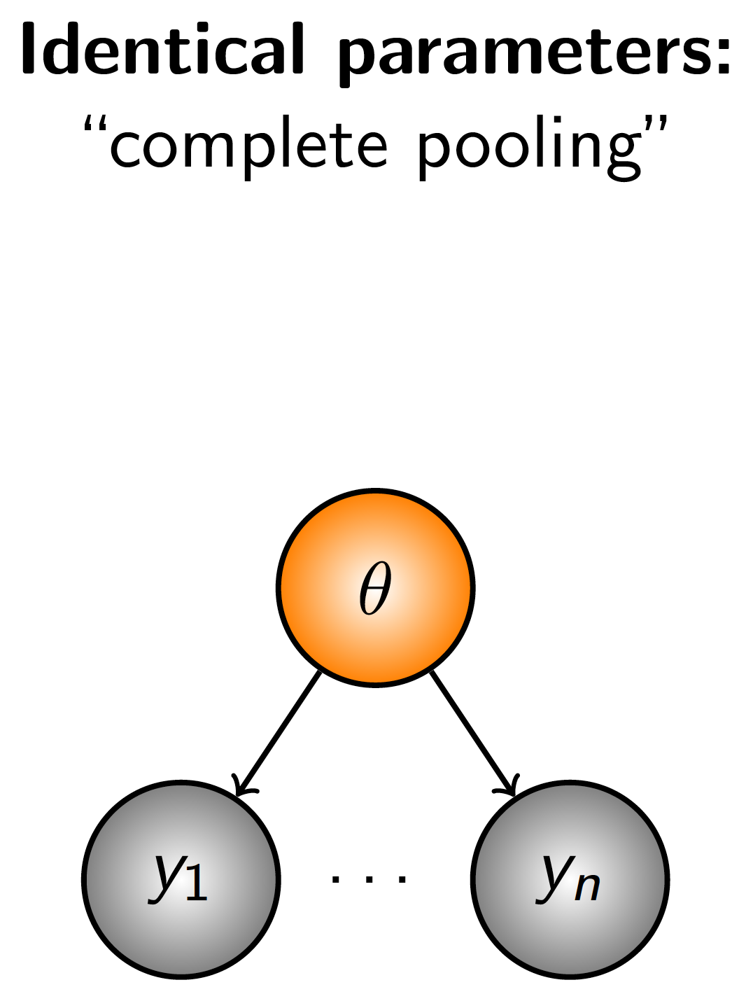
Figure 2.3: Diagrammatic representation complete pooling, a model structure in which all observations inform one parameter.
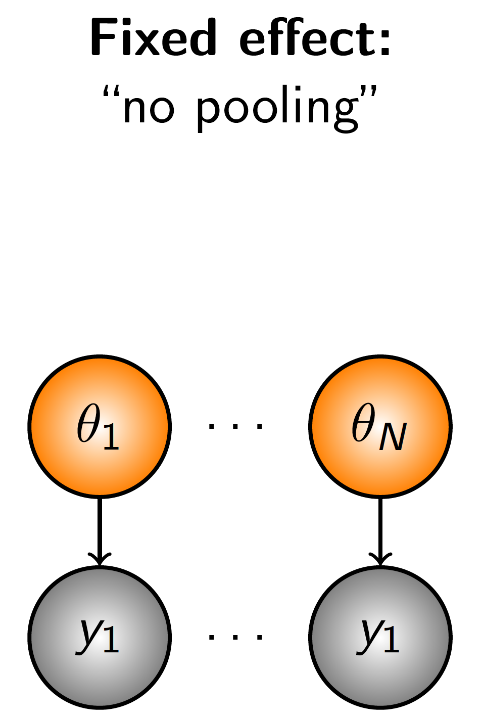
Figure 2.4: Diagrammatic representation no pooling, a model structure in which separate observations inform separate parameters.
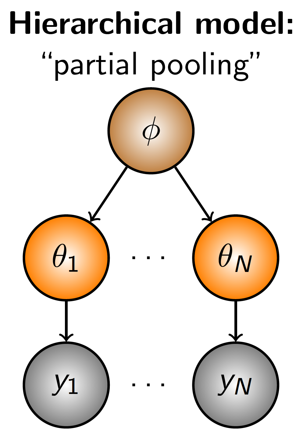
Figure 2.5: Diagrammatic representation partial pooling, a model structure in which different observations inform different latent parameters, which are then governed by additional parameters.
Example A simple example of rationalizing a hierarchical model might be modeling the size of birds. Our \(y\) values would be some measure of bird size. But we know that different species inherently attain different sizes; i.e., observations are not independent as any two size measurements from the same species are much more likely to be similar than to a measurement from an individual of another species). Therefore it makes sense to group the size observations by species, \(\theta_j\). However, we also know that there may still be relatedness among species, and as such some additional parameter, \(\phi\), can be added to govern the collection of species parameters. (To continue with the example, \(\phi\) might represnt a taxonomic order.)
Once you understand some examples of how hierarchical structures reflect the ecological systems we seek to model, you will find hierarchical models to be an often realistic representation of the system or process you want to understand—or at least more realistic than the traditional model representations.
2.3.1 Definitions of Hierarchical Models
There is a lot of terminology.
From Raudenbush and Bryk (2002)
- multilevel models in social research
- mixed-effects and random-effects models in biometric research
- random-coeffcient regression models in econometrics
- variance components models in statistics
- hierarchical models (Lindley and Smith 1972)
Some useful definitions are:
“…hierarchical structure, in which response variables are measured at the lowest level of the hierarchy and modeled as a function of predictor variables measured at that level and higher levels of the hierarchy.” Wagner, Hayes, and Bremigan (2006)
“Multilevel (hierarchical) modeling is a generalization of linear and generalized linear modeling in which regression coeffcients are themselves given a model, whose parameters are also estimated from data.” Gelman and Hill (2006)
“The existence of the process model is central to the hierarchical modeling view. We recognize two basic types of hierarchical models. First is the hierarchical model that contains an explicit process model, which describes realizations of an actual ecological process (e.g., abundance or occurrence) in terms of explicit biological quantities. The second type is a hierarchical model containing an implicit process model. The implicit process model is commonly represented by a collection of random effects that are often spatially and or temporally indexed. Usually the implicit process model serves as a surrogate for a real ecological process, but one that is diffcult to characterize or poorly informed by the data (or not at all).” Royle and Dorazio (2008)
“However, the term, hierarchical model, by itself is about as informative about the actual model used as it would be to say that I am using a four-wheeled vehicle for locomotion; there are golf carts, quads, Smartcars, Volkswagen, and Mercedes, for instance, and they all have four wheels. Similarly, plenty of statistical models applied in ecology have at least one set of random effects (beyond the residual) and therefore represent a hierarchical model. Hence, the term is not very informative about the particular model adopted for inference about an animal population.” Kéry and Schaub (2011)
References
Gelman, Andrew, and Jennifer Hill. 2006. Data Analysis Using Regression and Multilevel/Hierarchical Models. Cambridge university press.
Kéry, Marc. 2010. Introduction to Winbugs for Ecologists: Bayesian Approach to Regression, Anova, Mixed Models and Related Analyses. Academic Press.
Kéry, Marc, and Michael Schaub. 2011. Bayesian Population Analysis Using Winbugs: A Hierarchical Perspective. Academic Press.
Leslie, Paul W, and Michael A Little. 2003. “Human Biology and Ecology: Variation in Nature and the Nature of Variation.” American Anthropologist 105 (1). Wiley Online Library: 28–37.
Lindley, Dennis V, and Adrian FM Smith. 1972. “Bayes Estimates for the Linear Model.” Journal of the Royal Statistical Society: Series B (Methodological) 34 (1). Wiley Online Library: 1–18.
Raudenbush, Stephen W, and Anthony S Bryk. 2002. Hierarchical Linear Models: Applications and Data Analysis Methods. Vol. 1. Sage.
Royle, J Andrew, and Robert M Dorazio. 2008. Hierarchical Modeling and Inference in Ecology: The Analysis of Data from Populations, Metapopulations and Communities. Elsevier.
Wagner, Tyler, Daniel B Hayes, and Mary T Bremigan. 2006. “Accounting for Multilevel Data Structures in Fisheries Data Using Mixed Models.” Fisheries 31 (4). Taylor & Francis: 180–87.