Chapter 6 Survival Analysis
We turn our attention to survival analysis which deals with so-called time-to-event endpoints. To set the scene we will look at the lymphoma data and explain the basics of survival analysis. Then, we will discuss elastic net regularization in the context of cox regression, introduce the time-dependent Brier score as a measure of prediction accuracy, and we give an example on how to use the pec package to benchmark prediction algorithms.
6.1 Survival endpoints and Cox regression
We start by reading the lymphoma data which consists of gene expression data for \(p=7399\) genes measured on \(n=240\) patients, as well as survival data, for these patients.
# read gene expression matrix
x <- read.table("data/lymphx.txt")%>%
  as.matrix

# read survival data
y <- read.table("data/lymphtime.txt",header = TRUE)%>%
  as.matrix
The survival data consists of two variables time (the survival time) and status (event status, 1 in case of death, 0 in case of censoring).
| time | status |
|---|---|
| 5.0 | 0 |
| 5.9 | 0 |
| 6.6 | 0 |
| 13.1 | 0 |
| 1.6 | 1 |
| 1.3 | 1 |
The next plots shows the distribution of the survival times on a linear and log-scale.
The distribution on the left is right skewed. However, after a log transformation the distribution looks near-to-symmetric. What makes this endpoint so special? Why can’t we just use (regularized) linear regression to predict the (log) survival time based on the gene expression features? Such an approach would be shortsighted the reason being that we so far did not take into account the event status. The following graph shows survival times along side with the event status for a few patients. For patients with an event (blue triangles) the survival time equals the time-to-event. However, for censored patients (red dots) the actual time-to-event is not observed and will be larger than the survival time.
In survival analysis we denote time-to-event with \(T\). As illustrated above we typically only partially observe \(T\) as some subjects may be censored due to:
- Loss to follow-up
- Withdrawal from study
- No event by end of fixed study period.
Therefore we observe the survival time \(Y\) (which equals the event time or the censoring time whichever occurs earlier) and the event status \(D\) (\(D=1\) in case of event, \(D=0\) in case of censoring).
A fundamental quantity in survival analysis is the survival function
\[S(t)=P(T>t)=1-F(t)\]
which can be estimated using the Kaplan-Meier method. In R we use survfit and ggsurvplot to plot the Kaplan-Meier curve.
dat <- data.frame(y)
fit.surv <- survfit(Surv(time, status) ~ 1,
                    data = dat)
ggsurvplot(fit.surv,conf.int=FALSE)
## Warning: Using `size` aesthetic for lines was deprecated in ggplot2 3.4.0.
## ℹ Please use `linewidth` instead.
## ℹ The deprecated feature was likely used in the ggpubr package.
## Please report the issue at <https://github.com/kassambara/ggpubr/issues>.
## This warning is displayed once every 8 hours.
## Call `lifecycle::last_lifecycle_warnings()` to see where this warning was
## generated.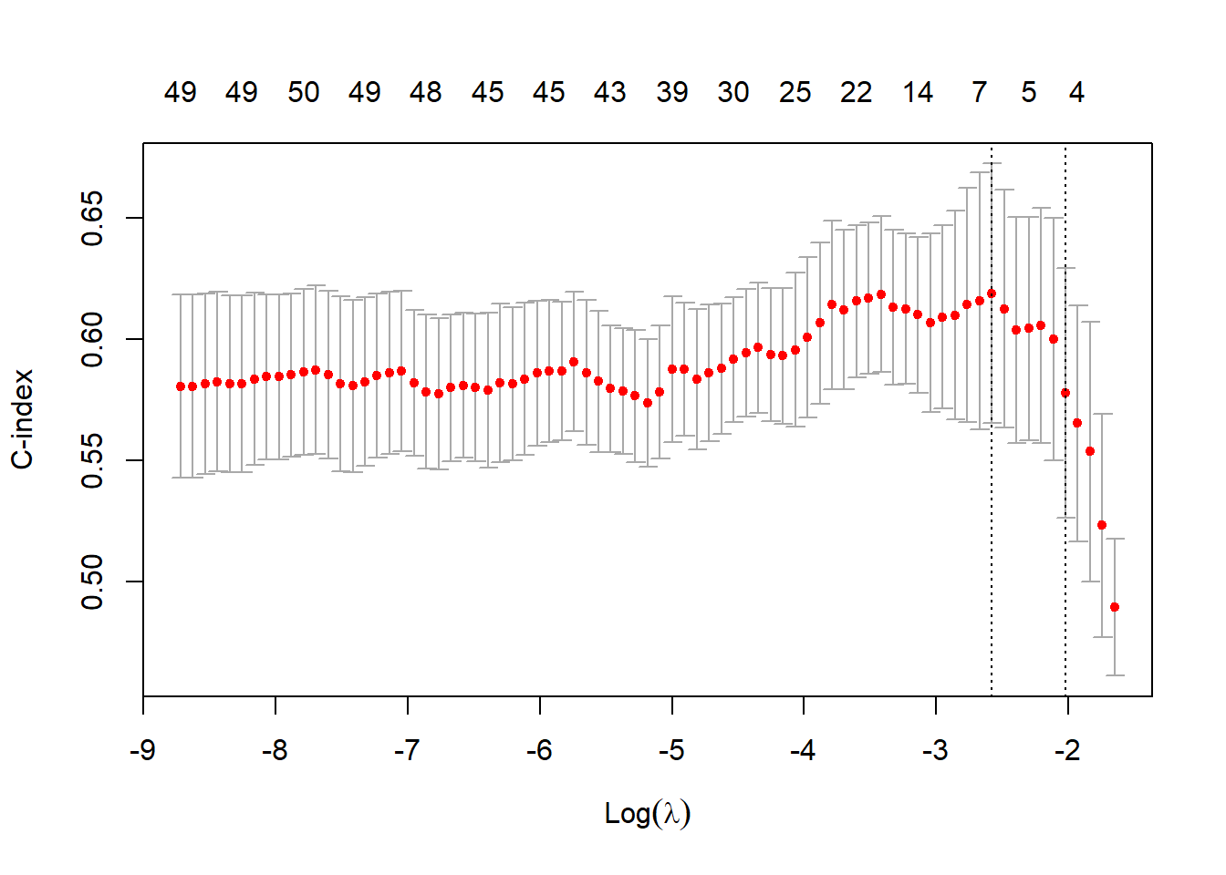
More specific information on the estimated survival probabilities can be obtained using the summary function.
# estimated probability of surviving beyond 10 years
summary(survfit(Surv(time, status) ~ 1, data = dat), times = 10)
Now, how do we study the relationship between covariates and survival time? The solution is Cox regression! We introduce the hazard function defined as
\[\begin{eqnarray*} h(t)&=&\lim_{dt\rightarrow 0}\frac{P(t\leq T < t+dt|T\geq t)}{dt}\\ &=&-S'(t)/S(t). \end{eqnarray*}\]
The Cox proportional hazards model then assumes a semi-parametric form for the hazard
\[h(t|X)=h_0(t)\exp(X^T\beta),\]
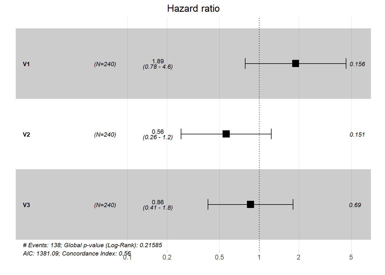
where \(h_0(t)\) is the baseline hazard and \(\beta\) are the regression coefficients. Cox regression estimates the regression coefficients by maximizing the so-called partial likelihood function (surprisingly this works without specifying the baseline hazard function). For illustration we fit a Cox regression model using the first 3 genes as predictors.
## Call:
## coxph(formula = Surv(time, status) ~ ., data = dat)
##
##   n= 240, number of events= 138
##
##       coef exp(coef) se(coef)      z Pr(>|z|)
## V1  0.6382    1.8931   0.4504  1.417    0.156
## V2 -0.5778    0.5611   0.4023 -1.436    0.151
## V3 -0.1508    0.8600   0.3785 -0.398    0.690
##
##    exp(coef) exp(-coef) lower .95 upper .95
## V1    1.8931     0.5282    0.7831     4.577
## V2    0.5611     1.7822    0.2551     1.234
## V3    0.8600     1.1627    0.4095     1.806
##
## Concordance= 0.559  (se = 0.028 )
## Likelihood ratio test= 4.46  on 3 df,   p=0.2
## Wald test            = 4.66  on 3 df,   p=0.2
## Score (logrank) test = 4.66  on 3 df,   p=0.2
The (exponentiated) regression coefficients are interpreted as hazard-ratios. For example a unit change in the 3rd covariate accounts for a risk reduction of \(\exp(\beta_3)\)=0.86 or \(14\%\). The results of Cox regression are often visualized using a forest plot.

6.2 Regularized Cox regression
The lymphoma data consists of \(p=\) 7399 predictors. A truly high-dimensional example! Similar as for linear- and logistic regression we can build upon the Cox regression model and use subset selection or regularization. The R package glmnet implements elastic net penalized cox regression. For illustration we restrict ourselves to the top genes (highest variance) and we scale the features as part of the data preprocessing.
# filter for top genes (highest variance) and scale the input matrix
topvar.genes <- order(apply(x,2,var),decreasing=TRUE)[1:50]
x <- scale(x[,topvar.genes])
We split the data set into training and test data.
set.seed(1234)
train_ind <- sample(1:nrow(x),size=nrow(x)/2)
xtrain <- x[train_ind,]
ytrain <- y[train_ind,]
xtest <- x[-train_ind,]
ytest <- y[-train_ind,]
We invoke glmnet with argument family="cox" and set the mixing parameter to \(\alpha=0.95\).
set.seed(1)
ytrain.surv <- Surv(ytrain[,"time"],ytrain[,"status"])
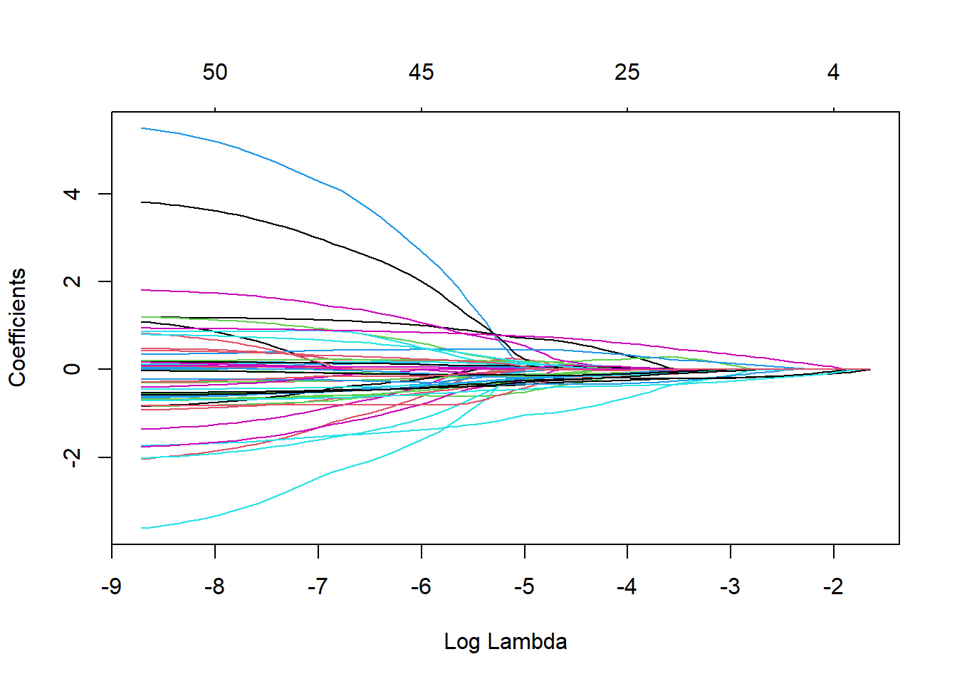
fit.coxnet <- glmnet(xtrain, ytrain.surv, family = "cox",alpha=0.95)
plot(fit.coxnet,xvar="lambda")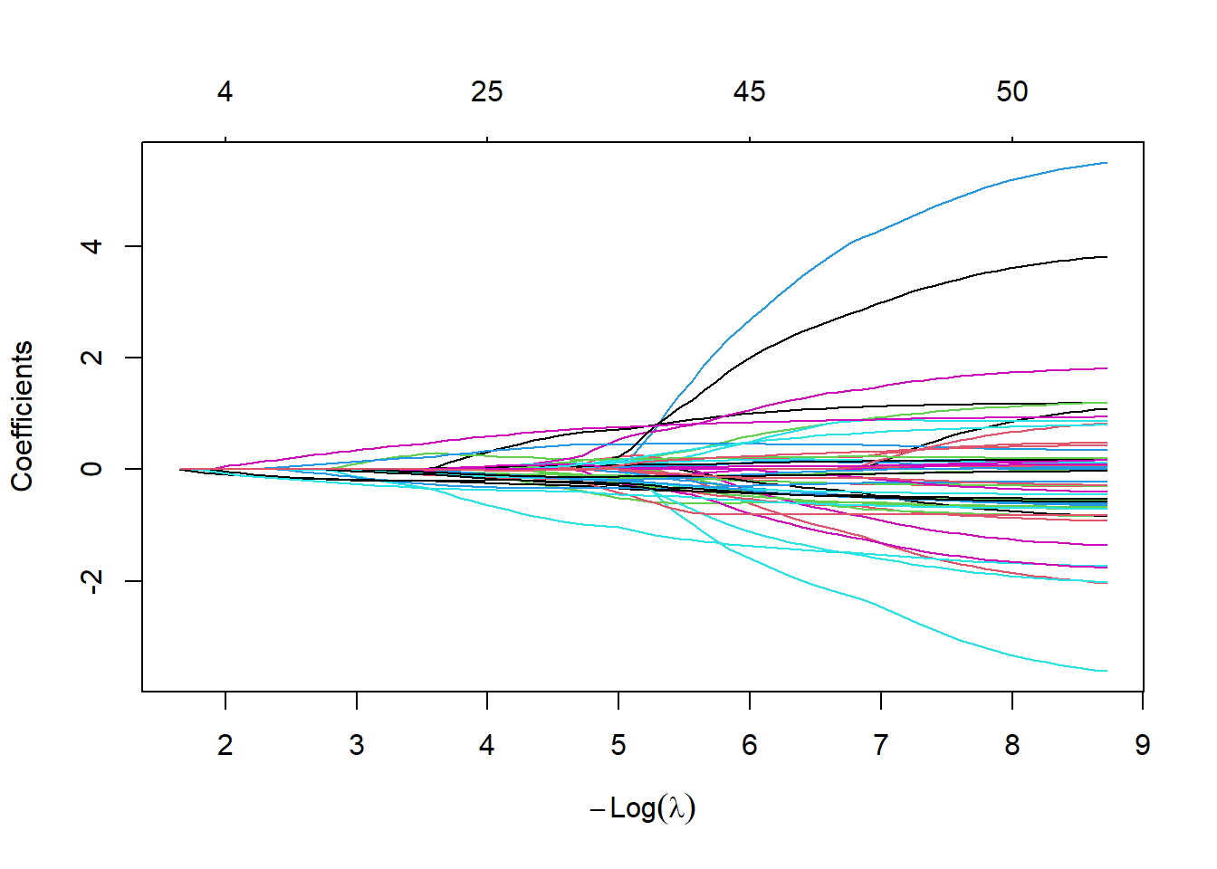
We tune the amount of penalization by using cross-validation and take Harrel’s concordance index as a goodness of fit measure.
cv.coxnet <- cv.glmnet(xtrain,ytrain.surv,
                       family="cox",
                       type.measure="C",
                       nfolds = 5,
                       alpha=0.95)
plot(cv.coxnet)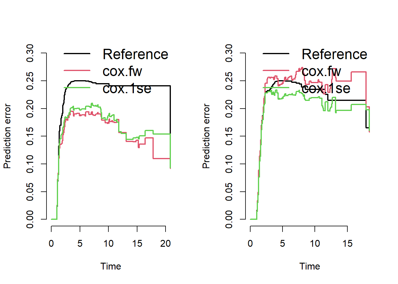
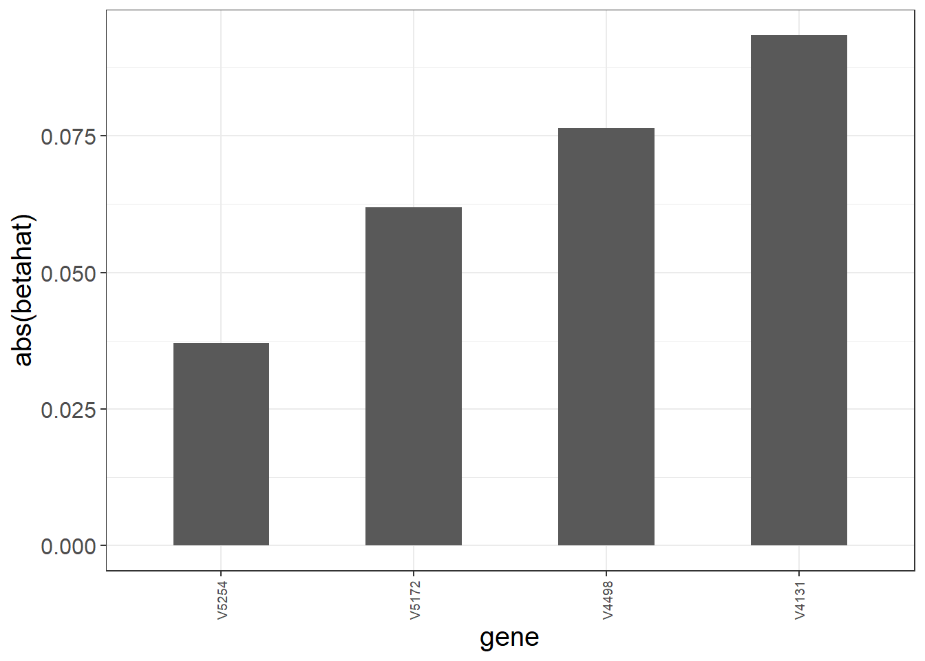
The C-index ranges from 0.5 to 1. A value of 0.5 indicates that the model is no better at predicting an outcome than random chance. The largest tuning parameter within 1se of the maximum C-index is \(\lambda_{\rm{opt}}=\) 0.132. The next graphic shows the magnitude of the non-zero coefficients (note that we standardized the input covariates).
We use the obtained model to make predictions on the test data. In particular we compute the linear predictor
\[\hat{f}(X_{\textrm{new}})=X_{\textrm{new}}^T\hat{\beta}_{\lambda_{\rm opt}}.\] We can now classify patients into good and poor prognosis based on thresholding the linear predictor at zero.
# linear predictor
lp <- predict(fit.coxnet,
              newx=xtest,
              s=cv.coxnet$lambda.1se,
              type="link")
dat.test <- data.frame(ytest)
dat.test$prognosis <- ifelse(lp>0,"poor","good")
fit.surv <- survfit(Surv(time, status) ~ prognosis,
                    data = dat.test)
ggsurvplot(fit.surv,conf.int = TRUE)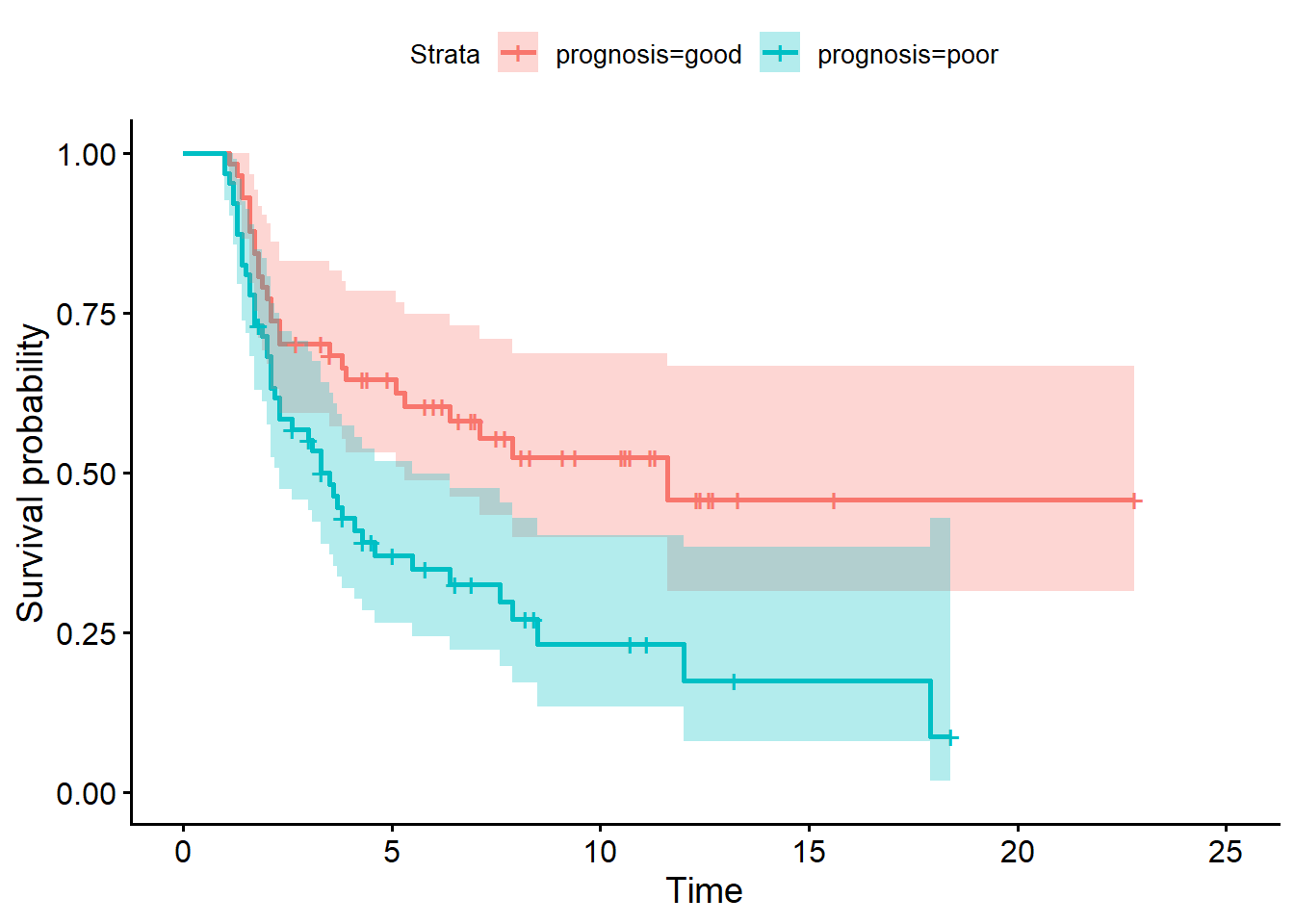
The survival curves are reasonably well separated, which suggests we have derived a gene signature which deserves further investigation.
6.3 Brier score
We have seen how to evaluate the generalization error in the linear regression and classification context. For time-to-event data this is slightly more involved. A popular way to quantify the prediction accuracy is the time-dependent Brier score
\[{\rm BS}(t,\hat{S})={\bf E}[(\Delta_{\rm{new}}(t)-\hat{S}(t|X_{\rm new}))^2] \]
where \(\Delta_{\textrm{new}}(t)={\bf 1}(T_{\textrm{new}}\geq t)\) is the true status of a new test subject and
\(\hat{S}(t|X_{\rm new})\) is the predicted survival probability. Calculation of the Brier score is complicated by the fact that we do not always observe the event time \(T\) due to censoring. The R package pec estimates the Brier score using a technique called Inverse Probability of Censoring Weighting (IPCW).
We use forward selection on the training data to obtain a prediction model.
dtrain <- data.frame(cbind(ytrain,xtrain))
dtest <- data.frame(cbind(ytest,xtest))
lo <- coxph(Surv(time,status)~1,data=dtrain,
            x=TRUE,y=TRUE)
up <- as.formula(paste("~",
                       paste(colnames(xtrain),
                             collapse="+")))
fit.fw <- stepAIC(lo,
                  scope=list(lower=lo,
                             upper=up),
                  direction="both",
                  trace=FALSE)
The following table summarizes the variables added in each step of the forward selection approach.
| Step | Df | Deviance | Resid. Df | Resid. Dev | AIC |
|---|---|---|---|---|---|
| NA | NA | 67 | 587.326 | 587.326 | |
| + V4131 | 1 | 7.554 | 66 | 579.771 | 581.771 |
| + V4498 | 1 | 7.405 | 65 | 572.366 | 576.366 |
| + V5172 | 1 | 5.272 | 64 | 567.094 | 573.094 |
| + V5254 | 1 | 7.388 | 63 | 559.706 | 567.706 |
| + V5223 | 1 | 3.802 | 62 | 555.903 | 565.903 |
| + V4356 | 1 | 3.766 | 61 | 552.138 | 564.138 |
| + V4341 | 1 | 3.311 | 60 | 548.826 | 562.826 |
We further run a Cox regression model based on the predictors selected by glmnet.
beta.1se <- coef(fit.coxnet,s=cv.coxnet$lambda.1se)
vars.1se <- rownames(beta.1se)[as.numeric(beta.1se)!=0]
fm.1se <- as.formula(paste0("Surv(time,status)~",
                            paste0(vars.1se,collapse="+")))
fit.1se <- coxph(fm.1se,data=dtrain,x=TRUE,y=TRUE)
Finally we use the pec package to calculate Brier scores for both models on the training and test data.
library(pec)
fit.pec.train <- pec::pec(
  object=list("cox.fw"=fit.fw,
              "cox.1se"=fit.1se),
  data = dtrain,
  formula = Surv(time, status) ~ 1,
  splitMethod = "none")


fit.pec.test <- pec::pec(
  object=list("cox.fw"=fit.fw,
              "cox.1se"=fit.1se),
  data = dtest,
  formula = Surv(time, status) ~ 1,
  splitMethod = "none")
The following figures show the Brier scores evaluated on training and test data.
The plot on the right indicates a slightly improved performance of the glmnet-selected-model over the reference model (no covariates, Kaplan-Meier estimate only).
The pec package can also be used to benchmark different prediction models. We illustrate this based on forward selection and random forest. In this illustration we do not split the data into training and test. Instead we use cross-validation to compare the two prediction approaches.
We start by writing a small wrapper function to use forward selection in pec. (A detailed description on the pec package and on how to set up wrapper functions is provided here.)
selectCoxfw <- function(formula,data,steps=100,direction="both")
{
  require(prodlim)
  fmlo <- reformulate("1",formula[[2]])
  fitlo <- coxph(fmlo,data=data,x=TRUE,y=TRUE)
  fwfit <- stepAIC(fitlo,
                   scope=list(lower=fitlo,
                              upper=formula),
                   direction=direction,
                   steps=steps,
                   trace=FALSE)
  if (fwfit$formula[[3]]==1){
    newform <- reformulate("1",formula[[2]])
    newfit <- prodlim(newform,
                      data=data)
  }else{
    newform <-fwfit$formula
    newfit <- coxph(newform,data=data,x=TRUE,y=TRUE)
  }
  out <- list(fit=newfit,
              In=attr(terms(newfit$formula),which = "term.labels"))
  out$call <-match.call()
  class(out) <- "selectCoxfw"

  out
}

predictSurvProb.selectCoxfw <- function(object,newdata,times,...){
  predictSurvProb(object[[1]],newdata=newdata,times=times,...)
}
We run forward selection.
dat <- data.frame(cbind(y,x))
fm <- as.formula(paste("Surv(time, status) ~ ",
                       paste(colnames(dat[,-(1:2)]),
                             collapse="+")))
fit.coxfw <- selectCoxfw(fm,data=dat,
                         direction="forward")
Then, we fit a random forest using cforest from the party package
and obtain the variable importance using the function varimp.
##
## Variable importance for survival forests; this feature is _experimental_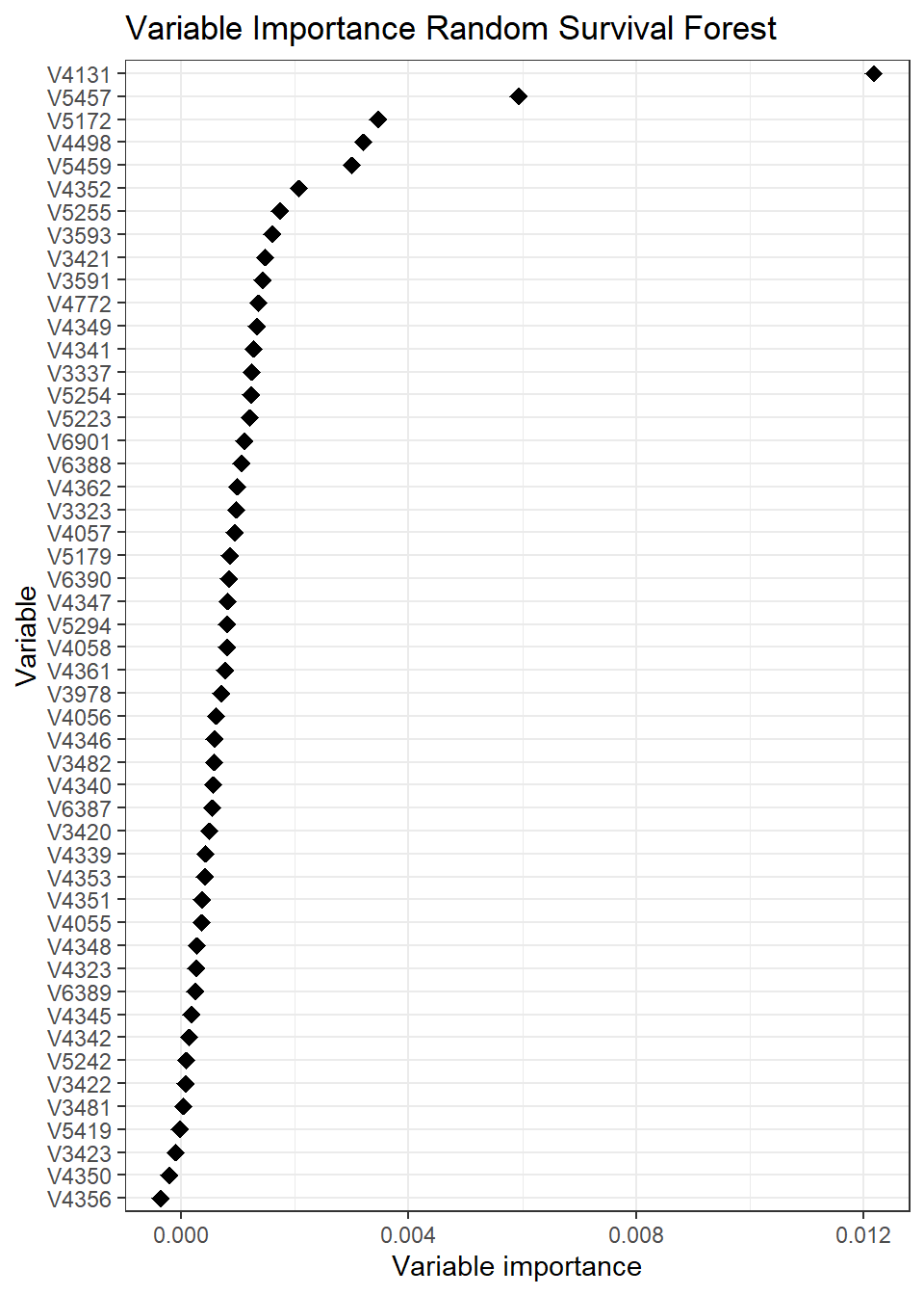
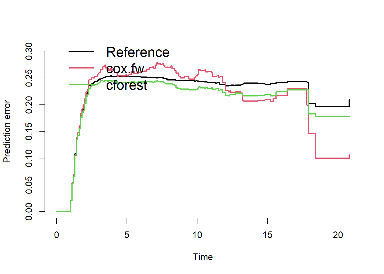
Finally, we compare the two models using the cross-validated Brier score.
pec.cv <- pec::pec(
  object=list("cox.fw"=fit.coxfw,"cforest"=fit.cforest),
  data = dat,
  formula = Surv(time, status) ~ 1,
  splitMethod = "cv5")
plot(pec.cv)
We conclude that forward selection and random forest do not outperform the reference model.