Chapter 4 Lasso Regression and Elasticnet
We have discussed Ridge regression and discussed its properties. Although Ridge regression can deal with high-dimensional data a disadvantage compared to subset- and stepwise regression is that it does not perform variable selection and therefore the interpretation of the final model is more challenging.
In Ridge regression we minimize \(\rm RSS(\beta)\) given constraints on the so-called L2-norm of the regression coefficients
\[\|\beta\|^2_2=\sum_{j=1}^p \beta^2_j \leq c.\]
Another very popular approach in high-dimensional statistics is Lasso regression (Lasso=least absolute shrinkage and selection operator). The Lasso works similarly. The only difference is that constraints are imposed on the L1-norm of the coefficients
\[\|\beta\|_1=\sum_{j=1}^p |\beta_j| \leq c.\]
Therefore the Lasso is referred to as L1 regularization. The change in the form of the constraints (L2 vs L1) has important implications. Figure 4.1 illustrates the geometry of the Lasso optimization. Geometrically the Lasso constraint is a diamond with “corners” (the Ridge constraint is a circle). If the residual sum of squares “hits” one of these corners then the coefficient corresponding to the axis is shrunk to zero. As \(p\) increases, the multidimensional diamond has an increasing number of corners, and so it is highly likely that some coefficients will be set to zero. Hence, the Lasso performs not only shrinkage but it also sets some coefficients to zero, in other words the Lasso simultaneously performs variable selection. A disadvantage of the “diamond” geometry is that in general there is no closed form solution for the Lasso (the Lasso optimisation problem is not differentiable at the corners of the diamond).
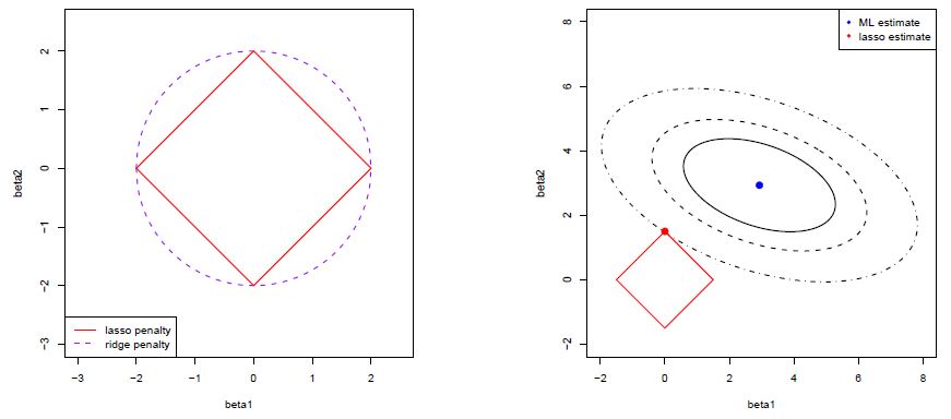
Figure 4.1: Geometry of Lasso regression.
Similar to Ridge regression the Lasso can be formulated as a penalisation problem
\[ \hat{\beta}^{\rm Lasso}_{\lambda}=\text{arg}\min\limits_{\beta}\;\textrm{RSS}(\beta)+\lambda\|\beta\|_1. \]
To fit the Lasso we use glmnet (with \(\alpha=1\)).
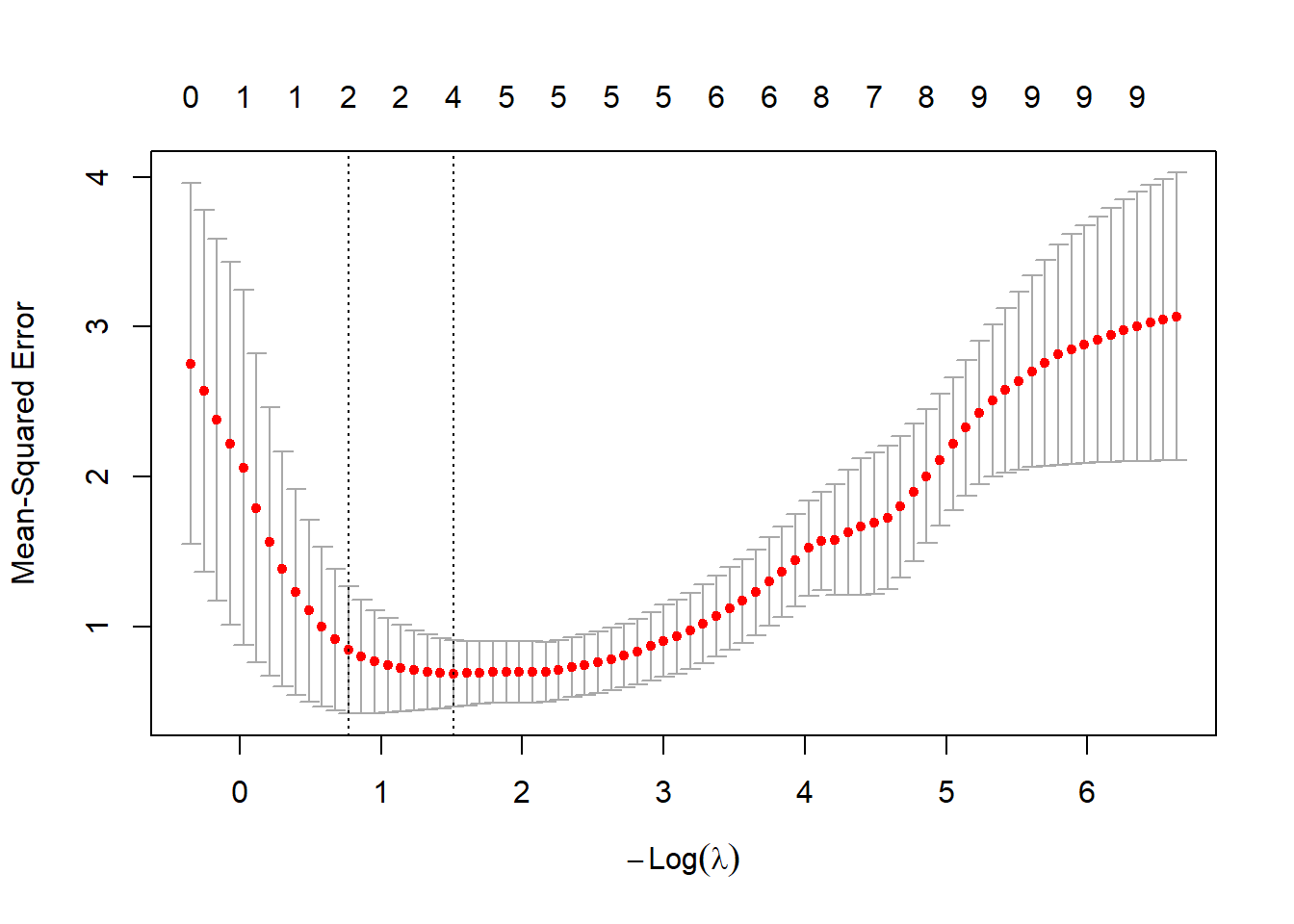
The following figure shows the Lasso solution for a grid of \(\lambda\) values. We note that the Lasso shrinks some coefficients to exactly zero. The number of active covariates (i.e., the number of non-zero coefficients) is indicated at the top of the graph.

We choose the optimal tuning parameter \(\lambda_{\rm opt}\) by cross-validation.
## [1] 0.2201019The coefficient for the optimal model can be extracted using the coef function.
beta.lasso <- coef(fit.lasso.glmnet, s = cv.lasso.glmnet$lambda.min)
names(beta.lasso) <- colnames(xtrain)
beta.lasso
## 10 x 1 sparse Matrix of class "dgCMatrix"
## s=0.2201019
## (Intercept) 0.08727244
## V1 1.44830414
## V2 -0.04302609
## V3 .
## V4 -0.07325330
## V5 .
## V6 .
## V7 .
## V8 -0.24778236
## V9 .We now discuss some properties of the Lasso.
4.1 Numerical optimization and soft thresholding
In general there is no closed-form solution for the Lasso. The optimization has to be performed numerically. An efficient algorithm is implemented in glmnet and is referred to as “Pathwise Coordinate Optimization”. The algorithm updates one regression coefficient at a time using the so-called soft-thresholding function. This is done iteratively until some convergence criterion is met.
An exception is the case with an orthonormal design matrix \(\bf X\), i.e. \(\bf X^T\bf X=\bf I\). Under this assumption we have
\[\begin{align*} \textrm{RSS}(\beta)&=(\textbf{y}-\textbf{X}\beta)^T(\textbf{y}-\textbf{X}\beta)\\ &=\textbf{y}^T\textbf{y}-2\beta^T\hat\beta^{\rm OLS}+\beta^T\hat\beta \end{align*}\]
and therefore the Lasso optimization reduces to \(j=1,\ldots,p\) univariate problems
\[\textrm{minimize}\; -\hat\beta_j^{\rm OLS}\beta_j+0.5\beta_j^2+0.5\lambda |\beta_j|.\]
In the exercises we will show that the solution is
\[\begin{align*} \hat{\beta}_{\lambda,j}^{\textrm{Lasso}}&=\textrm{sign}(\hat{\beta}_j^{\rm OLS})\left(|\hat{\beta}_j^{\rm OLS}|-0.5\lambda\right)_{+}\\ &=\left\{\begin{array}{ll} \hat\beta^{\rm OLS}_j-0.5\lambda & {\rm if}\;\hat\beta^{\rm OLS}_j>0.5\lambda\\ 0 & {\rm if}\;|\hat\beta^{\rm OLS}_j|\leq 0.5\lambda\\ \hat\beta^{\rm OLS}_j+0.5\lambda & {\rm if}\;\hat\beta^{\rm OLS}_j<-0.5\lambda \end{array} \right. \end{align*}\]
That is, in the orthonormal case, the Lasso is a function of the OLS estimator. This function, depicted in the next figure, is referred to as soft-thresholding.
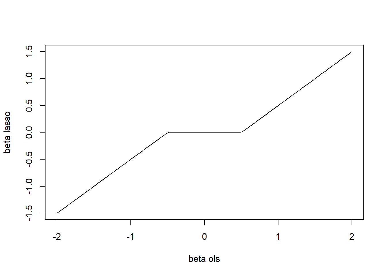
Figure 4.2: Soft-thresholding function.
The soft-thresholding function is not only used for numerical optimization of the Lasso but also plays a role in wavelet thresholding used for signal and image denoising.
4.2 Variable selection
We have seen that the Lasso simultaneously shrinks coefficients and sets some of them to zero. Therefore the Lasso performs variable selection which leads to more interpretabel models (compared to Ridge regression). For the Lasso we can define the set of selected variables
\[\hat S^{\rm Lasso}_{\lambda}=\{j\in (1,\ldots,p); \hat\beta^{\rm Lasso}_{\lambda,j}\neq 0\}\]
In our example this set can be obtained as follows.
## [1] "(Intercept)" "V1" "V2" "V4" "V8"An interesting question is whether the Lasso does a good or bad job in variable selection. That is, does \(\hat S^{\rm Lasso}_{\lambda}\) tend to agree with the true set of active variables \(S_0\)? Or, does the Lasso typically under- or over-select covariates? These questions are an active field of statistical research.
4.3 Elasticnet regression
We have encountered the L1 and L2 penalty. The Lasso (L1) penalty has the nice property that it leads to sparse solutions, i.e. it simultaneously performs variable selection. A disadvantage is that the Lasso penalty is somewhat indifferent to the choice among a set of strong but correlated variables. The Ridge (L2) penalty, on the other hand, tends to shrink the coefficients of correlated variables toward each other. An attempt to take the best of both worlds is the elastic net penalty which has the form
\[\lambda \Big(\alpha \|\beta\|_1+(1-\alpha)\|\beta\|_2^2\Big).\]
The second term encourages highly correlated features to be averaged, while the first term encourages a sparse solution in the coefficients of these averaged features.
In glmnet the elastic net regression is implemented using the mixing parameter \(\alpha\). The default is \(\alpha=1\), i.e. the Lasso.
4.4 P-values for high-dimensional regression
The Lasso is a very effective method in the \(p>>n\) context. It avoids overfitting by shrinking the regression coefficients and eases interpretation by simultaneously performing variable selection. The Lasso has inspired many researchers which developed new statistical methods. One such approach uses the Lasso combined with the idea of “sample splitting” to obtain p-values in the high-dimensional regression context. The method consists of the following steps:
- Sample splitting: Randomly divide the data into two parts, the in- and out-sample.
- Screening: Use the Lasso to identify the key variables \(\hat S^{\rm Lasso}_{\lambda}\) (based on the in- sample)
- P-value calculation: Obtain p-values using OLS regression on the selected variables \(\hat S^{\rm Lasso}_{\lambda}\) (based on the out-sample)
The p-values obtained in step 3 are sensitive to the random split chosen in step 1. Therefore, in order to avoid a “p-value lottery”, the steps 1-3 are repeated many times and the results are aggregated. For more details we refer to Meinshausen and Bühlmann (2009). The approach is implemented in the R package hdi.
4.5 Diabetes example
We now review what we have learned with an example. The data that we consider consist of observations on 442 patients, with the response of interest being a quantitative measure of disease progression one year after baseline. There are ten baseline variables — age, sex, body-mass index, average blood pressure, and six blood serum measurements — plus quadratic terms, giving a total of \(p=64\) features. The task for a statistician is to construct a model that predicts the response \(Y\) from the covariates. The two hopes are, that the model would produce accurate baseline predictions of response for future patients, and also that the form of the model would suggest which covariates were important factors in disease progression.
We start by splitting the data into training and test data.
set.seed(007)
data <- readRDS(file="data/diabetes.rds")
train_ind <- sample(seq(nrow(data)),size=nrow(data)/2)
data_train <- data[train_ind,]
xtrain <- as.matrix(data_train[,-1])
ytrain <- data_train[,1]
data_test <- data[-train_ind,]
xtest <- as.matrix(data_test[,-1])
ytest <- data_test[,1]
We perform forward stepwise regression.
# Full model
fit.full <- lm(y~.,data=data_train)

# Forward regression
fit.null <- lm(y~1,data=data_train)
fit.fw <- stepAIC(fit.null,direction="forward",
                  scope=list(lower=fit.null,
                             upper=fit.full

                  ),
                  trace = FALSE
)
The selection process is depicted in the following table.
| Step | Df | Deviance | Resid. Df | Resid. Dev | AIC |
|---|---|---|---|---|---|
| NA | NA | 220 | 1295012.8 | 1919.37 | |
| + ltg | 1 | 480436.38 | 219 | 814576.4 | 1818.91 |
| + bmi | 1 | 90618.04 | 218 | 723958.3 | 1794.85 |
| + map | 1 | 39190.49 | 217 | 684767.8 | 1784.55 |
+ glu^2 |
1 | 32560.95 | 216 | 652206.9 | 1775.78 |
| + hdl | 1 | 17629.79 | 215 | 634577.1 | 1771.72 |
| + sex | 1 | 24729.23 | 214 | 609847.9 | 1764.94 |
| + age.sex | 1 | 10928.14 | 213 | 598919.7 | 1762.94 |
| + sex.ldl | 1 | 12011.61 | 212 | 586908.1 | 1760.47 |
| + glu | 1 | 7553.66 | 211 | 579354.5 | 1759.60 |
| + bmi.map | 1 | 6805.57 | 210 | 572548.9 | 1758.99 |
| + map.glu | 1 | 10462.13 | 209 | 562086.8 | 1756.92 |
The regression coefficients and the corresponding statistics of the AIC-optimal model are shown next.
| term | estimate | std.error | statistic |
|---|---|---|---|
| (Intercept) | 152.74 | 3.54 | 43.13 |
| ltg | 506.51 | 97.36 | 5.20 |
| bmi | 351.03 | 90.31 | 3.89 |
| map | 399.67 | 90.07 | 4.44 |
glu^2 |
278.25 | 89.96 | 3.09 |
| hdl | -271.94 | 85.48 | -3.18 |
| sex | -240.93 | 84.40 | -2.85 |
| age.sex | 166.79 | 75.08 | 2.22 |
| sex.ldl | -152.53 | 71.14 | -2.14 |
| glu | 148.03 | 90.65 | 1.63 |
| bmi.map | 193.57 | 86.01 | 2.25 |
| map.glu | -196.91 | 99.84 | -1.97 |
We continue by fitting Ridge regression. We show the trace plot and the cross-validation plot.
# Ridge
set.seed(1515)
fit.ridge <- glmnet(xtrain,ytrain,alpha=0)
fit.ridge.cv <- cv.glmnet(xtrain,ytrain,alpha=0)
plot(fit.ridge,xvar="lambda")
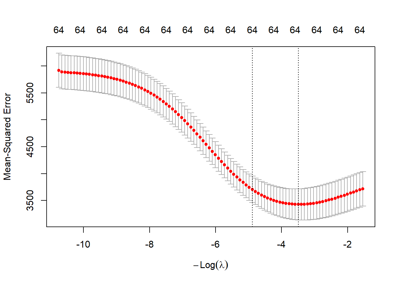
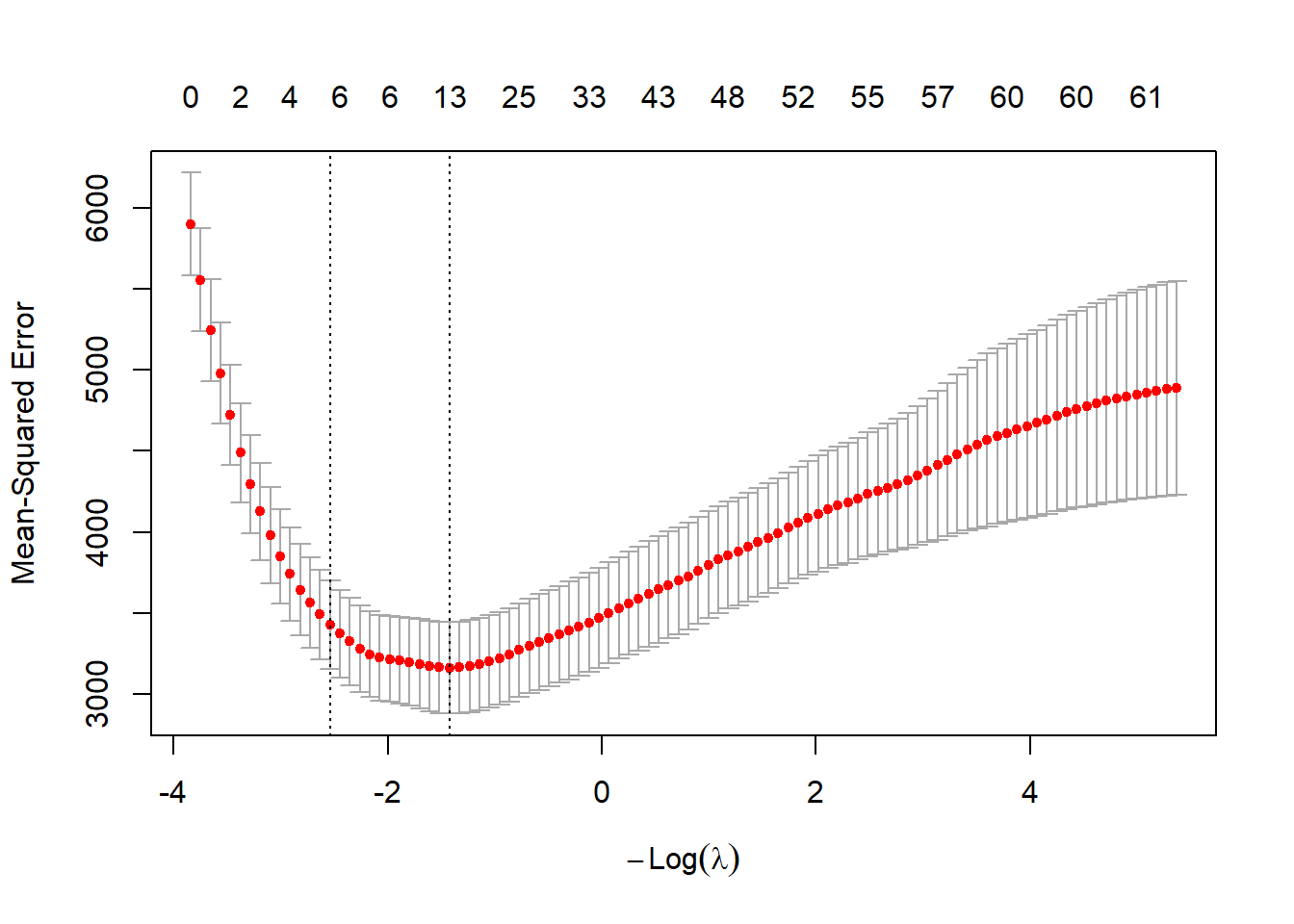
Finally, we run the Lasso approach and show the trace and the cross-validation plots.
# Lasso
set.seed(1515)
fit.lasso <- glmnet(xtrain,ytrain,alpha=1)
fit.lasso.cv <- cv.glmnet(xtrain,ytrain,alpha=1)
plot(fit.lasso,xvar="lambda")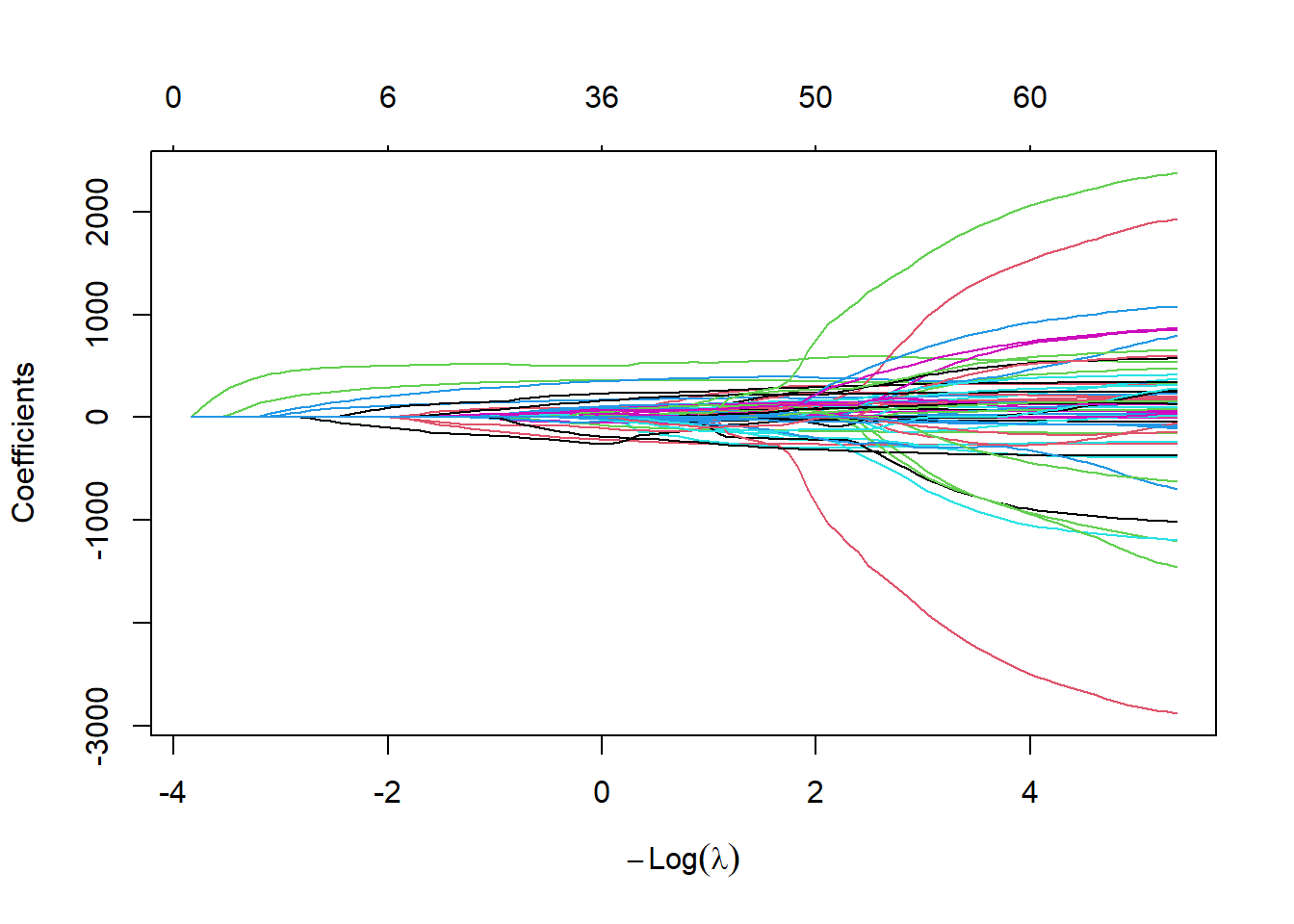
We calculate the root-mean-square errors (RMSE) on the test data and compare with the full model.
# RMSE
pred.full <- predict(fit.full,newdata=data_test)
pred.fw <- predict(fit.fw,newdata=data_test)
pred.ridge <- as.vector(predict(fit.ridge,newx=xtest,s=fit.ridge.cv$lambda.1se))
pred.lasso <- as.vector(predict(fit.lasso,newx=xtest,s=fit.lasso.cv$lambda.1se))
res.rmse <- data.frame(
  method=c("full","forward","ridge","lasso"),
  rmse=c(RMSE(pred.full,ytest),RMSE(pred.fw,ytest),
         RMSE(pred.ridge,ytest),RMSE(pred.lasso,ytest)))
kable(res.rmse,digits = 2,
booktabs=TRUE)| method | rmse |
|---|---|
| full | 81.90 |
| forward | 55.64 |
| ridge | 60.62 |
| lasso | 59.64 |
The Lasso has the lowest generalization error (RMSE). We plot the regression coefficients for all 3 methods.
beta.fw <- coef(fit.fw)
beta.ridge <- coef(fit.ridge,s=fit.ridge.cv$lambda.1se)
beta.lasso <- coef(fit.lasso,s=fit.lasso.cv$lambda.1se)
res.coef <- data.frame(forward=0,ridge=as.numeric(beta.ridge),
                       lasso=as.numeric(beta.lasso))
rownames(res.coef) <- rownames(beta.ridge)
res.coef[names(beta.fw),"forward"] <- beta.fw
res.coef$coef <- rownames(res.coef)
res.coef.l <- pivot_longer(res.coef,cols=c("forward","ridge","lasso"),
                           names_to="method")

res.coef.l%>%
  dplyr::mutate(coef=factor(coef,levels = unique(coef)))%>%
  ggplot(.,aes(x=coef,y=value,fill=method))+
  geom_bar(width=0.5,position = position_dodge(width = 0.8),stat="identity")+
  theme_bw()+
  theme(legend.position = "top",
        axis.text.x = element_text(angle = 90,vjust = 0.5, hjust=1))+
  scale_fill_grey(aesthetics = c("fill","color"))+
  xlab("")+ylab("beta")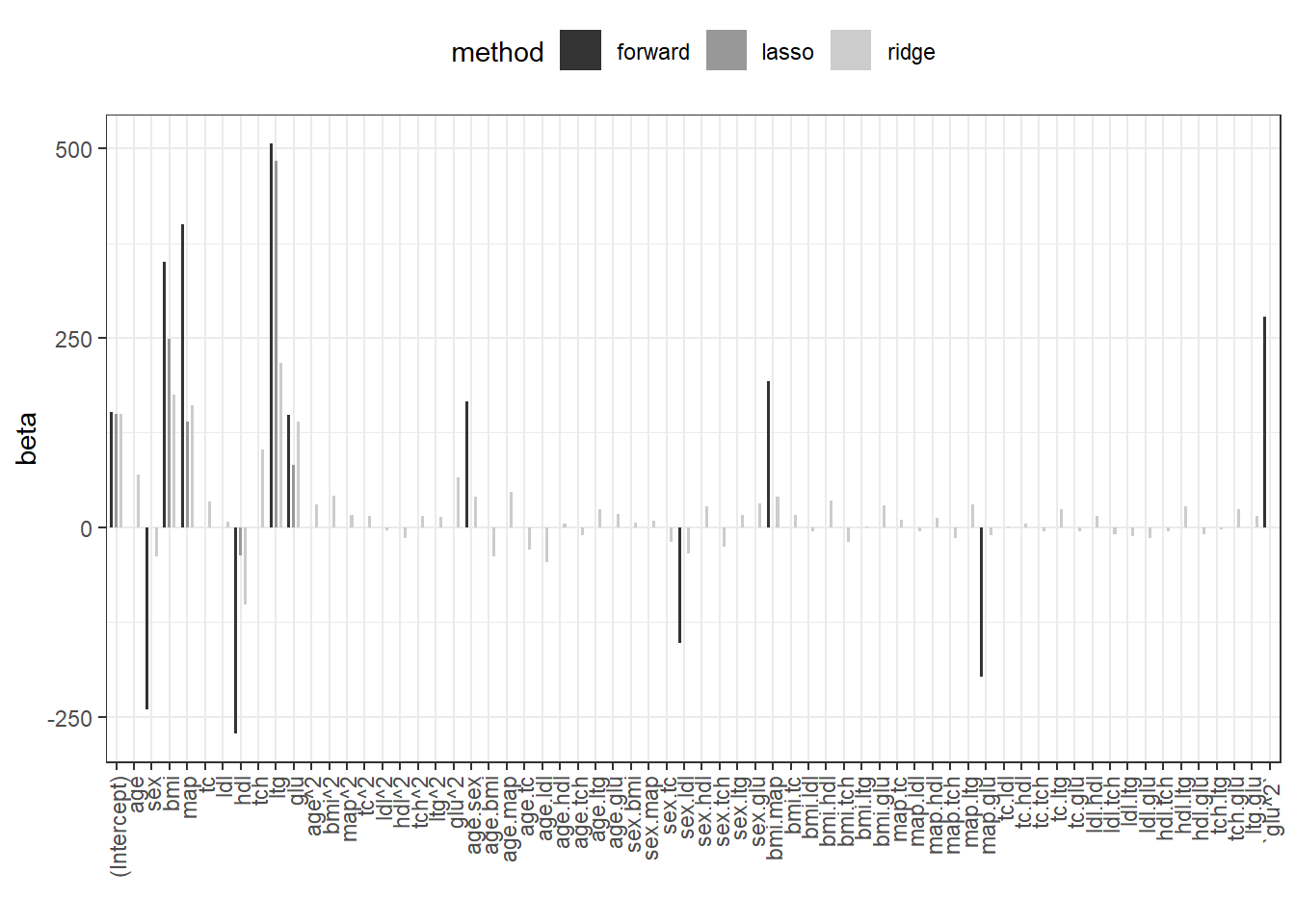
We point out that the same analysis can be conducted with the caret package. The code to do so is provided next.
## Setup trainControl: 10-fold cross-validation
tc <- trainControl(method = "cv", number = 10)

## Ridge
lambda.grid <- fit.ridge.cv$lambda
fit.ridge.caret<-train(x=xtrain,
                       y=ytrain,
                       method = "glmnet",
                       tuneGrid = expand.grid(alpha = 0,
                                              lambda=lambda.grid),
                       trControl = tc
)

# CV curve
plot(fit.ridge.caret)
# Best lambda
fit.ridge.caret$bestTune$lambda
# Model coefficients
coef(fit.ridge.caret$finalModel,fit.ridge.cv$lambda.1se)%>%head
# Make predictions
fit.ridge.caret %>% predict(xtest,s=fit.ridge.cv$lambda.1se)%>%head

## Lasso
lambda.grid <- fit.lasso.cv$lambda
fit.lasso.caret<-train(x=xtrain,
                       y=ytrain,
                       method = "glmnet",
                       tuneGrid = expand.grid(alpha = 1,
                                              lambda=lambda.grid),
                       trControl = tc
)

# CV curve
plot(fit.lasso.caret)
# Best lambda
fit.lasso.caret$bestTune$lambda
# Model coefficients
coef(fit.lasso.caret$finalModel,
     fit.lasso.caret$bestTune$lambda)%>%head
# Make predictions
fit.lasso.caret%>%predict(xtest,
                          s=fit.ridge.cv$lambda.1se)%>%head

## Compare Ridge and Lasso
models <- list(ridge= fit.ridge.caret,lasso = fit.lasso.caret)
resamples(models) %>% summary( metric = "RMSE")