Chapter 5 Classification

Our high-dimensional considerations so far focused on the linear regression model. We now extend this to classification.

5.1 Logistic regression

We start with standard logistic regression where the response \(Y\) takes values \(0\) and \(1\), and the aim is to do prediction based on covariates \(X=(X_1,\ldots,X_p)\). We model the probability of success (i.e., \(Y=1\)) \[p(x;\beta)=P(Y=1|X=x;\beta)\] assuming a binomial distribution with logit link function

\[\text{logit}(x;\beta)=\log \Big(\frac{p(x;\beta)}{1-p(x;\beta)}\Big)=X^T\beta.\]

In logistic regression we estimate the regression parameter \(\beta\) by maximizing the log-likelihood

\[\begin{align*} \ell(\beta|\textbf{y},\textbf{X})&=\sum_{i=1}^{n}(1-y_i)\log(1-p(x_i;\beta))+y_i\log p(x_i;\beta)\\ &=\sum_{i=1}^{n}y_i x_i^T\beta - \log(1+\exp(x_i^T\beta)). \end{align*}\]

Given an estimate \(\hat \beta\) (from training data), prediction based on new input data \(X_{\rm new}\) can be obtained via the predicted probability of success \(p(X_{\rm new};\hat \beta)\), e.g. the class labels corresponding to the maximum probability

\[\begin{align*} \hat{Y}\equiv\hat{G}(X_{\textrm{new}})\equiv\left\{ \begin{array}{ll} 1, & \mbox{if $p(X_{\textrm{new}};\hat\beta)>0.5$}.\\ 0, & \mbox{otherwise}. \end{array} \right. \end{align*}\]

There are different measures to judge the quality of the predictions. We focus on the misclassification error which is simply the fraction of misclassified test samples. Another important measure used in the context of classification is the receiver operating characteristic (ROC).

We illustrate logistic regression using an example taken from the book by Hastie, Tibshirani, and Friedman (2001). The data shown in Figure 5.1 are a subset of the Coronary Risk-Factor Study (CORIS) baseline survey, carried out in three rural areas of the Western Cape, South Africa. The aim of the study was to establish the intensity of ischemic heart disease risk factors in that high-incidence region. The data represent white males between 15 and 64, and the response variable is the presence or absence of myocardial infarction (MI) at the time of the survey (the overall prevalence of MI was 5.1% in this region). There are 160 cases in our data set, and a sample of 302 controls. The variables are:

• sbp: systolic blood pressure
• tobacco: cumulative tobacco (kg)
• ldl: low densiity lipoprotein cholesterol adiposity
• famhist: family history of heart disease (Present, Absent)
• obesity
• alcohol: current alcohol consumption
• age: age at onset
• chd: response, coronary heart disease.

We start by drawing scatter plots of pairs of risk factors and by color coding cases and controls.

dat <- readRDS(file="data/sahd.rds")
pairs(data.matrix(dat[,-1]),
      col=ifelse(dat$chd==1,"red","blue"),
      pch=ifelse(dat$chd==1,1,2))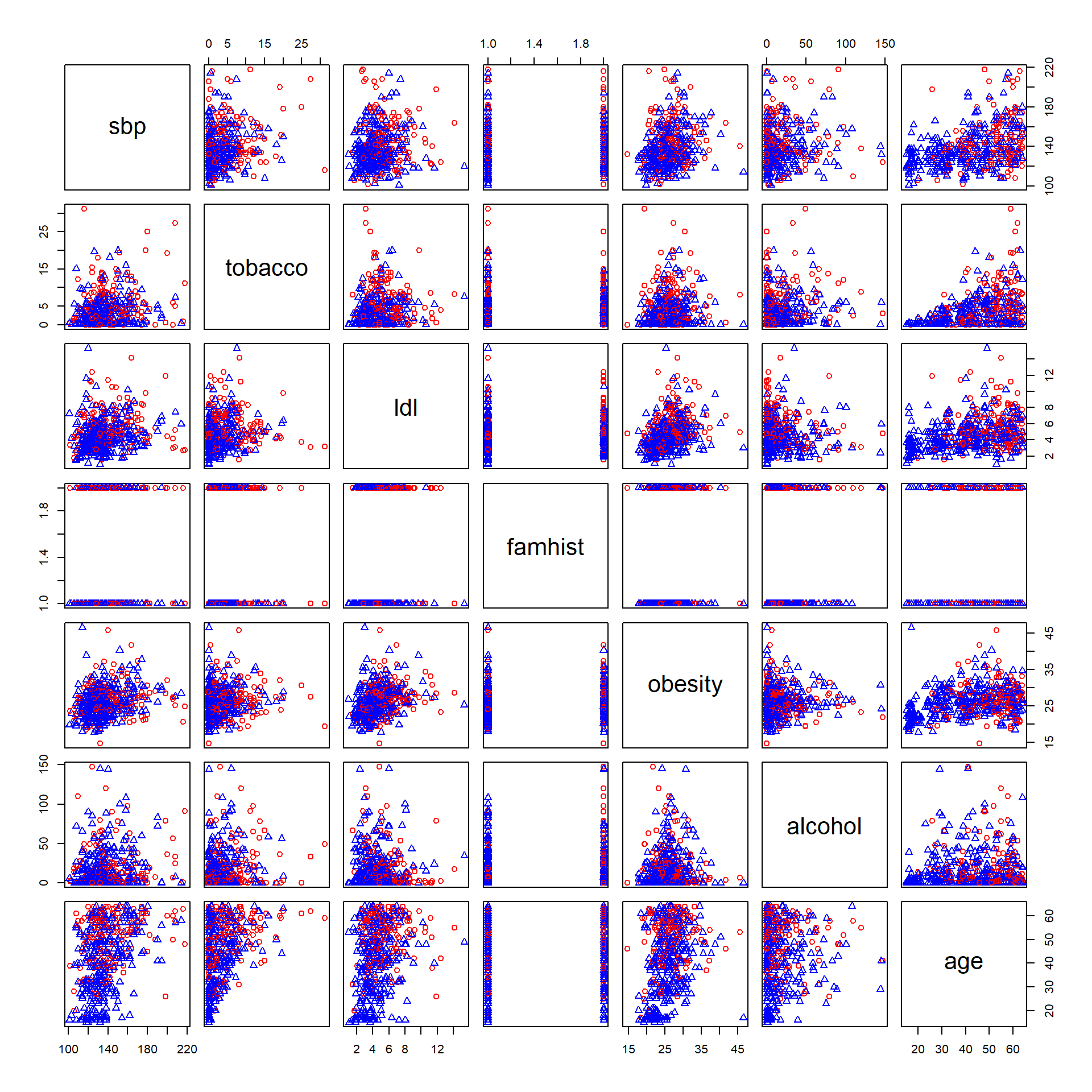

Figure 5.1: Pairs plot of South African Heart Disease Data (red circles: cases, blue triangles: controls).

Next, we fit a logistic regression model using the function glm.

fit.logistic <- glm(chd~sbp+tobacco+ldl+famhist+obesity+alcohol+age,
                    data=dat,
                    family="binomial")
kable(broom::tidy(fit.logistic),digits=3,booktabs=TRUE)

term	estimate	std.error	statistic	p.value
(Intercept)	-4.130	0.964	-4.283	0.000
sbp	0.006	0.006	1.023	0.306
tobacco	0.080	0.026	3.034	0.002
ldl	0.185	0.057	3.219	0.001
famhistPresent	0.939	0.225	4.177	0.000
obesity	-0.035	0.029	-1.187	0.235
alcohol	0.001	0.004	0.136	0.892
age	0.043	0.010	4.181	0.000

There are some surprises in this table of coefficients, which must be interpreted with caution. Systolic blood pressure (sbp) is not significant! Nor is obesity, and its sign is negative. This confusion is a result of the correlation between the set of predictors. On their own, both sbp and obesity are significant, and with positive sign. However, in the presence of many other correlated variables, they are no longer needed (and can even get a negative sign).

How does one interpret a coefficient of \(0.080\) (Std. Error = \(0.026\)) for tobacco, for example? Tobacco is measured in total lifetime usage in kilograms, with a median of \(1.0\)kg for the controls and \(4.1\)kg for the cases. Thus an increase of 1kg in lifetime tobacco usage accounts for an increase in the odds of coronary heart disease of \(\exp(0.080)\)=1.083 or \(8.3\)%. Incorporating the standard error we get an approximate \(95\)% confidence interval of \(\exp(0.081 ± 2 × 0.026)\)=(1.035,1.133).

5.2 Regularized logistic regression

Similar as for linear regression, in the high-dimensional setting where \(n\) is small compared to \(p\), the maximum likelihood estimator does lead to overfitting and a poor generalisation error. In the context of linear regression we introduced regularization by imposing constraints on the regression coefficients. It is easy to generalize this idea to logistic regression. In R subset- and stepwise logistic regression is implemented in stepAIC and elastic net regularization in glmnet (with argument family="binomial"). In the latter case the algorithm optimizes the negative log-likelihood penalized with the elastic net term:

\[\begin{align*} \hat{\beta}^{\rm EN}_{\alpha,\lambda}&=\text{arg}\min\limits_{\beta}\;-\frac{1}{n}\ell(\beta|{\bf y},{\bf X})+\lambda\big(\alpha\|\beta\|_1+(1-\alpha)\|\beta\|_2^2/2\big). \end{align*}\]

With \(\alpha=0\) and \(\alpha=1\) we obtain the Ridge and the Lasso solution, respectively.

We turn back to the heart disease example and perform backward stepwise logistic regression.

fit.bw <- stepAIC(fit.logistic,direction = "backward",trace=FALSE)

The terms removed in each step are provided in the next table.

kable(as.data.frame(fit.bw$anova),digits=3,booktabs=TRUE)

Step	Df	Deviance	Resid. Df	Resid. Dev	AIC
	NA	NA	454	483.174	499.174
- alcohol	1	0.019	455	483.193	497.193
- sbp	1	1.104	456	484.297	496.297
- obesity	1	1.147	457	485.444	495.444

The regression coefficients of the final model are shown below.

kable(broom::tidy(fit.bw),digits=3,booktabs=TRUE)

term	estimate	std.error	statistic	p.value
(Intercept)	-4.204	0.498	-8.437	0.000
tobacco	0.081	0.026	3.163	0.002
ldl	0.168	0.054	3.093	0.002
famhistPresent	0.924	0.223	4.141	0.000
age	0.044	0.010	4.521	0.000

We continue with the Lasso approach and show the trace plot.

x <- scale(data.matrix(dat[,-1]))
y <- dat$chd
fit.lasso <- glmnet(x=x,y=y,family="binomial")
plot(fit.lasso,xvar = "lambda",label=TRUE)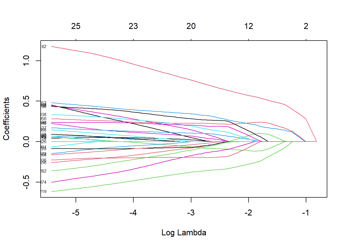

The first coefficient which is shrunk to zero is alcohol followed by sbp and obesity. This is in line with the results from backward selection.

Let’s now turn to a truly high-dimensional example. The data consists of expression levels recorded for \(3'571\) genes in \(72\) patients with leukemia. The binary outcome encodes the disease subtype: acute lymphobastic leukemia (ALL) or acute myeloid leukemia (AML). The data are represented as a 72 x 3,571 matrix \(\bf X\) of gene expression values, and a vector \(\bf y\) of 72 binary disease outcomes. We first create training and test data.

# set seed
set.seed(15)

# get leukemia data
leukemia <- readRDS(file="data/leukemia.rds")
x <- leukemia$x
y <- leukemia$y

# test/train 
ind_train <- sample(1:length(y),size=length(y)/2)
xtrain <- x[ind_train,]
ytrain <- y[ind_train]
xtest <- x[-ind_train,]
ytest <- y[-ind_train]

The following heatmap illustrates the gene expression values for the different patients.

We now run the elastic net logistic regression approach and make a trace plot

# run glmnet
alpha  <- 0.95                # elastic net mixing parameter.
fit.glmnet <-glmnet(xtrain,ytrain,family = "binomial",alpha=alpha)
plot(fit.glmnet,xvar="lambda",label=TRUE)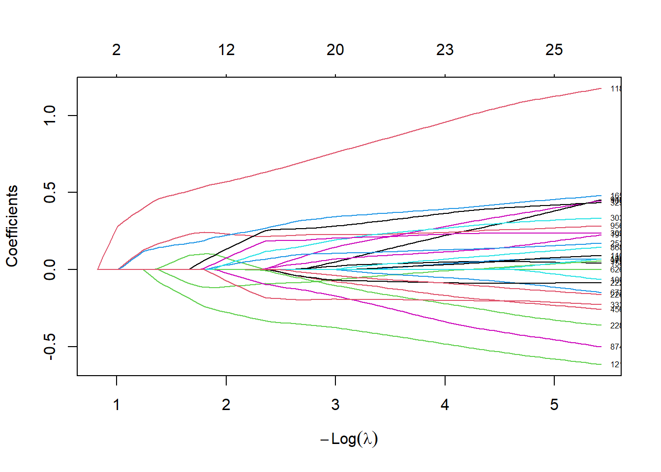

We perform 10-fold cross-validation and plot the misclassification error.

set.seed(118)
# run cv.glmnet
nfolds <- 10 # number of cross-validation folds.
cv.glmnet <- cv.glmnet(xtrain,ytrain,
                       family = "binomial",type.measure = "class",
                       alpha = alpha,nfolds = nfolds)
plot(cv.glmnet)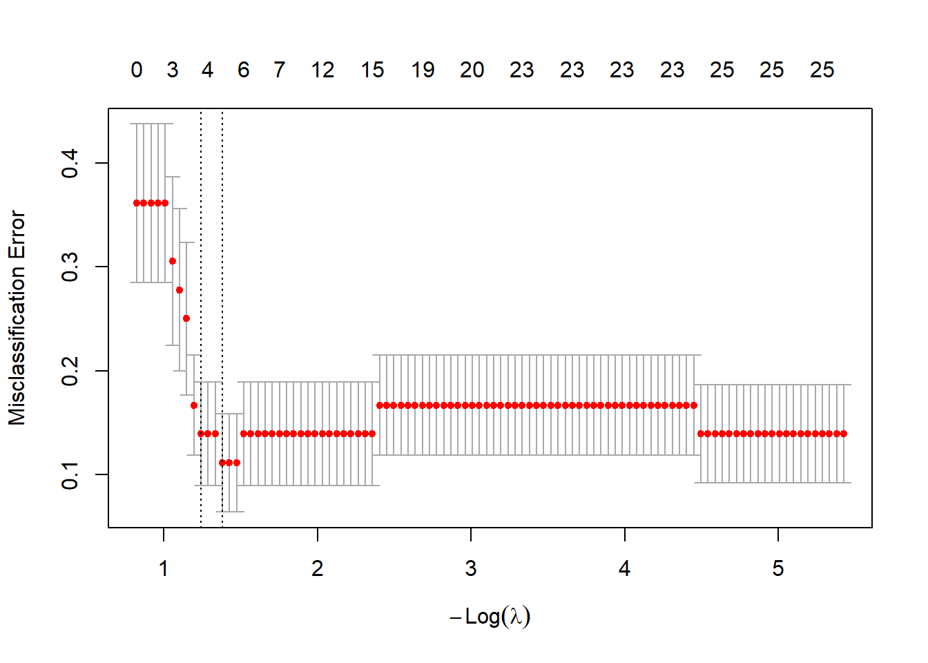

We take lambda.1se as the optimal tuning parameter

#sum(coef(fit.glmnet, s = cv.glmnet$lambda.1se)!=0)
#sum(coef(fit.glmnet, s = cv.glmnet$lambda.min)!=0)
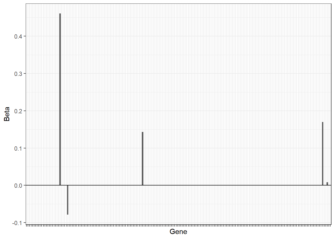
(lambda.opt <- cv.glmnet$lambda.1se)

## [1] 0.2891844

and visualize the size of the coefficients using a barplot

beta.glmnet <- coef(fit.glmnet, s = cv.glmnet$lambda.min)
df <- data.frame(Gene=paste0("G",1:(length(beta.glmnet)-1)),
                 Beta=as.numeric(beta.glmnet)[-1])
df%>%
  arrange(desc(abs(Beta)))%>%
  slice(1:200)%>%
  ggplot(.,aes(x=Gene,y=Beta))+
  geom_bar(stat="identity")+
  theme_bw()+
  theme(axis.text.x = element_blank())+
  geom_hline(yintercept = 0)

Finally, we predict the disease outcome of the test samples using the fitted model and compare against the observed outcomes of the test samples.

pred <- c(predict(fit.glmnet,xtest,s = lambda.opt,type = "class"))
print(table(true = factor(ytest),pred = factor(pred)))

##     pred
## true  0  1
##    0 24  0
##    1  3  9

The misclassification error on the test data can be calculated as follows.

round(mean(pred!=ytest),3)

## [1] 0.083

5.3 Classification trees

Classification is a frequent task in data mining and besides logistic regression there is a variety of other methods developed for this task. We first introduce classification trees which learn a binary tree where leaves represent class labels and branches represent conjunctions of features that lead to those class labels. The package rpart can be used to learn classification trees.

# load packages
library(rpart)
library(rpart.plot)

# read south african heart disease data
dat <- readRDS(file="data/sahd.rds")

# grow a classification tree
fit.tree <- rpart(chd~.,data=dat,method="class")
# plot(fit.tree, uniform=TRUE)
# text(fit.tree, use.n=TRUE, all=TRUE, cex=.8)
rpart.plot(fit.tree,extra=1,under=TRUE,tweak = 1.2,faclen=3)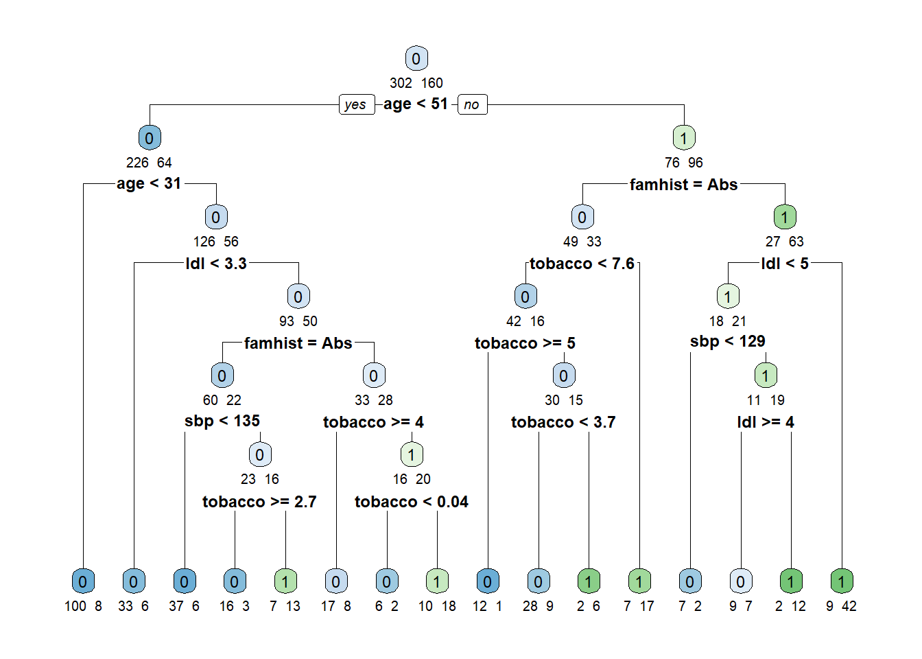

The algorithm starts by growing a typically too large tree which overfits the data. The next step is to “prune” the tree to obtain a good trade-off between goodness of fit and complexity. The following plot shows the relative cross-validation error (relative to the trivial tree consisting of only the root node) as a function of the complexity parameter.

plotcp(fit.tree,cex.lab=1.5,cex.axis=1.2,cex=1.5)

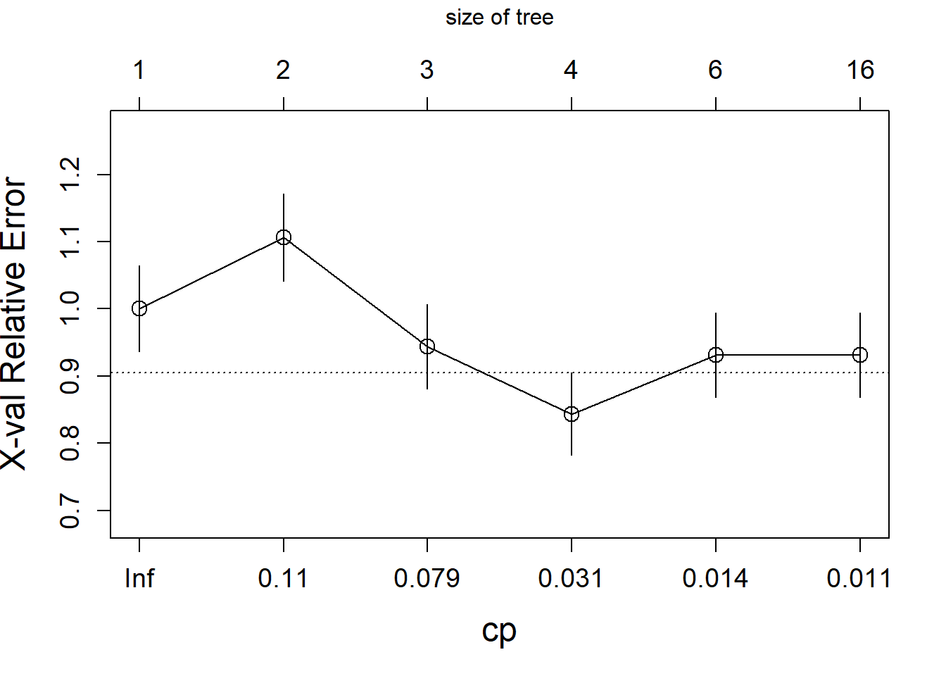
The optimally pruned tree has size 4 (i.e., 4 leave nodes).

# prune the tree
fit.prune<- prune(fit.tree, 
                  cp=fit.tree$cptable[which.min(fit.tree$cptable[,"xerror"]),"CP"])
rpart.plot(fit.prune,extra=1)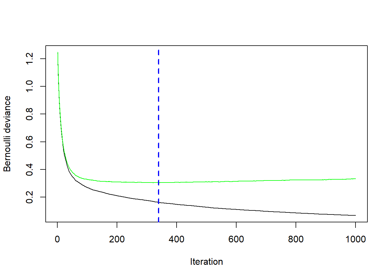

Classification trees are the basis of powerful Machine Learning (ML) algorithms, namely Random Forest and AdaBoost.M1. Both methods share the idea of growing various trees and combining the outputs to obtain a more powerful classification. However, the two approaches differ in the way they grow the trees and in how they do the aggregation. Random Forest works by building trees based on bootstrapped data sets and by aggregating the results using a majority vote (see Figure 5.2). The key idea behind AdaBoost.M1 is to sequentially fit a “stump” (i.e., a tree with two leaves) to weighted data with repeatedly modified weights. The weights assure that each stump takes the errors made by the previous stump into account. In that way a sequence of weak classifiers \(\{G_m\}_{m=1}^M\) is produced and finally a powerful new classifier is obtained by giving more influence towards the more accurate classifiers (see Figure 5.3).

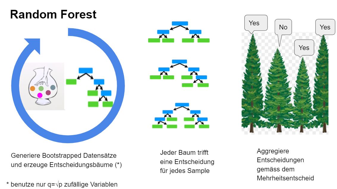
Figure 5.2: The key idea of Random Forest

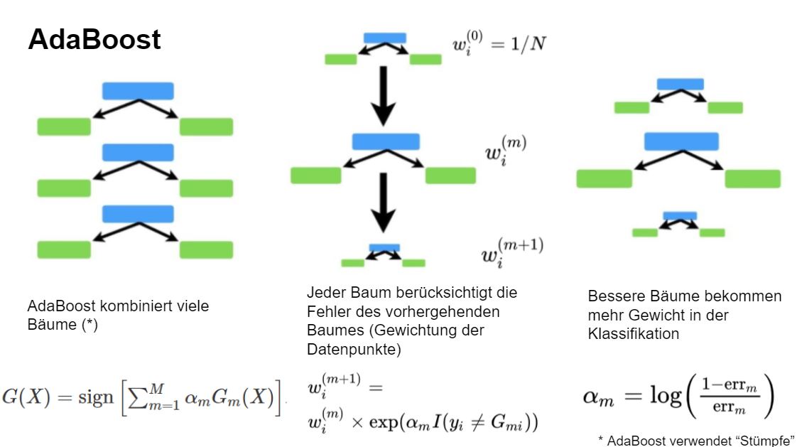
Figure 5.3: The key idea of AdaBoost

5.4 AdaBoost.M1

The following algorithm describes AdaBoost.M1:

1. Initialize the weights \(w_i=1/n\), \(i=1,\ldots,n\)
2. For \(m=1\) to \(M\):
   1. Fit a weak classifier \(G_m\) (a “stump”) to the training data using weights \(w_i\).
   2. Compute the weighted error rate \[{\rm err}_m=\frac{\sum_{i=1}^n w_i I(y_i\neq G_m(x_i))}{\sum_{i=1}^n w_i}.\]
   3. Compute \(\alpha_m=\log((1-{\rm err}_m)/{\rm err}_m)\)
   4. Update \(w_i\leftarrow w_i \exp(\alpha_m I(y_i\neq G_m(x_i)))\), \(i=1,2,...,n.\)
3. Output the combined classifier \(G(X)={\rm sign}\left[\sum_{m=1}^M \alpha_m G_m(X)\right]\).

In line 2d the weights are updated. Interestingly, the observations that where misclassified by \(G_{m}(x)\) receive a larger weight which forces the next classifier \(G_{m+1}(x)\) to focus on the misclassified observations. In line 3 the final predictor is assembled. The parameters \(\alpha_m\) balance the influence of the individual classifiers towards the more accurate classifiers in the sequence. AdaBoost can be viewed as special case of forward stagewise additive modeling. Let’s assume an additive model

\[f(x)=\sum_{m=1}^M \beta_m b(x;\gamma_m)\]

with basis function \(b(x,\gamma)\). Given a loss function \(L(y,f(x))\) such models can be fitted by minimizing a loss function,

\[\min_{\{\beta_m,\gamma_m\}} \sum_{i=1}^N L(y_i,\sum_{m=1}^{M}\beta_m b(x_i; \gamma_m)).\]

Forward stagewise modelling solves this optimization problem by sequentially adding new basis functions to the expansion without adjusting the parameters of those that have already been added, that is at the m-th iteration we obtain

\[ (\beta_m,\gamma_m)=\text{arg}\min\limits_{\beta,\gamma} \sum_{i=1}^N L(y_i,f_{m-1}(x_i)+\beta b(x_i; \gamma))\]

and update \[f_m(x)=f_{m-1}(x)+\beta_m b(x;\gamma_m).\] The following sketch shows that the m-th iteration of AdaBoost.M1 corresponds to forward stagewise modelling with exponential loss function and classification trees as basis functions:

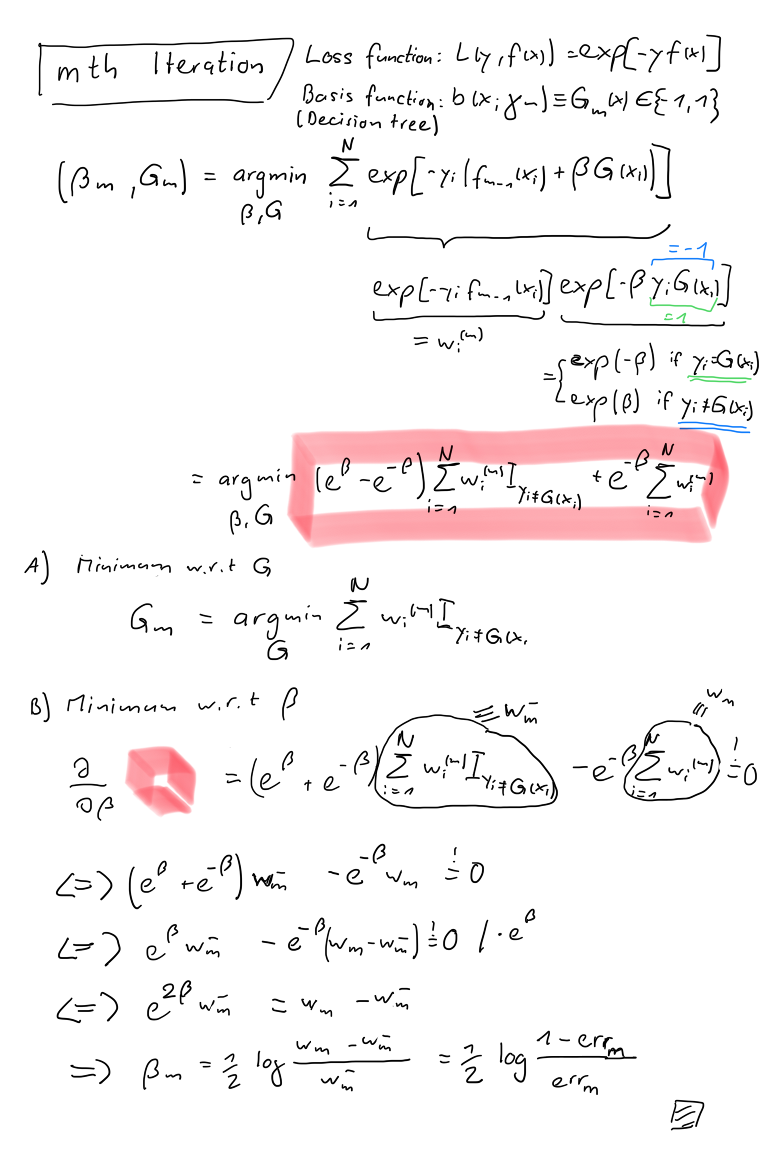
Figure 5.4: Forward stage-wise modelling and AdaBoost.M1.

5.5 Gradient Boosting

We have seen the connection between AdaBoost and forward stagewise modeling. We will look now into Gradient Boosting which generalizes this approach. Let’s assume an additive expansion of trees

\[f_M(x)=\sum_{m=1}^M T(x;\Theta_m)\]

where \(T(x;\Theta)\) is a regression tree of fixed size \(J\) (regression tree is a binary tree applied to a continuous response variable). In the m-th iteration of the forward stagewise algorithm we must solve

\[\Theta_m=\text{arg}\min\limits_{\Theta_m} \sum_{i=1}^N L(y_i,f_{m-1}(x_i)+T(x_i;\Theta_m))\]

and then update \[f_{m}(x)=f_{m-1}(x)+T(x;\Theta_m).\] In general, this is a very challenging optimization problem. Luckily, for the squared error loss the optimization simplifies to

\[\Theta_m=\text{arg}\min\limits_{\Theta_m} \sum_{i=1}^N \left(y_i-(f_{m-1}(x_i)+T(x_i;\Theta_m))\right)^2\]

and the solution is the regression tree which best predicts the residuals \[r_{im}=y_i-f_{m-1}(x_i).\] How does one solve the optimization problem for more general loss functions? It can be shown that the more general optimization problem can be approximated by solving the squared error problem but using pseudo residuals \[\tilde{r}_{im}=-\left[\frac{\partial L(y_i,f(x_i))}{\partial f(x_i)}\right]_{f=f_{m-1}}\] which correspond to the negative gradient of the loss function. Finally, it has been shown that the performance of gradient boosting can be further improved by updating

\[f_{m}(x)=f_{m-1}(x)+\nu \;T(x;\Theta_m)\]

where \(0<\nu<1\) is a shrinkage factor which “moderates” the contribution of the new tree \(T(x;\Theta_m)\) to the current approximation. Gradient boosting has three tuning parameters, namely, the number of boosting iterations (\(M\)), the shrinkage parameter (\(\nu\)), and the tree size (\(J\)). Typically, \(J = 6\), \(\nu = 0.1\), and \(M\) is chosen to reach the optimal generalization error.

Let’s illustrate Gradient Boosting using Email spam data. The data consists of information from 4601 email messages. The aim is to predict whether the email is spam. For all 4601 email messages, the true outcome (email type) “email” or “spam” is available, along with the relative frequencies of 57 of the most commonly occurring words and punctuation marks in the email message. This is a supervised learning problem, with the outcome the class variable email/spam. It’s also a classification problem.

# read email spam data
spam <- readRDS(file="data/spam.rds")

# training and test set
set.seed(102)
train <- sort(sample(nrow(spam),3065))
spam.train<- spam[train,]
spam.test<- spam[-train,]

We run Gradient Boosting gbm with distribution = "bernoulli" and tuning parameters \(\nu=0.1\) (shrinkage=0.1), \(J=4\) (interaction.depth=3) and \(M=1000\) (n.trees=1000).

library(gbm)
fit.boost <-gbm(spam~.,
                data=spam.train,
                distribution = "bernoulli",
                shrinkage=0.1,
                n.trees=1000,
                interaction.depth = 3,
                cv.folds=5) 
fit.boost

## gbm(formula = spam ~ ., distribution = "bernoulli", data = spam.train, 
##     n.trees = 1000, interaction.depth = 3, shrinkage = 0.1, cv.folds = 5)
## A gradient boosted model with bernoulli loss function.
## 1000 iterations were performed.
## The best cross-validation iteration was 340.
## There were 57 predictors of which 46 had non-zero influence.

In addition we perform 5-fold cross-validation (cv.folds=5) in order to monitor performance as a function of the boosting iterations.

# find index for n trees with minimum CV error
which.min(fit.boost$cv.error)

## [1] 340

# plot loss as a function of the number of boosting iteration
gbm.perf(fit.boost, method = "cv")

## [1] 340

References

Hastie, Trevor, Robert Tibshirani, and Jerome Friedman. 2001. The Elements of Statistical Learning. Springer Series in Statistics. New York, NY, USA: Springer New York Inc.