Chapter 7 High-Dimensional Feature Assessment

A frequent task is to find features which differ with respect to one or more experimental factors. We illustrate this type of analysis using a gene expression experiment (\(p=15923\) genes) performed with \(12\) randomly selected mice from two strains. The features are the \(p=15923\) genes and the strain (A vs B) is the experimental factor.

A commonly used format for gene expression data is the ExpressionSet class from the Biobase package. The actual expressions are retrieved using the function exprs. Information on the phenotypes is obtained using pData and with fData we get more information on the genes (“features”).

We load the ExpressionSet.

esetmouse <- readRDS(file="data/esetmouse.rds")
class(esetmouse)

## [1] "ExpressionSet"
## attr(,"package")
## [1] "Biobase"

dim(esetmouse)

## Features  Samples 
##    15923       24

We can look at the expression values of the first sample and the first 6 genes.

exprs(esetmouse)[1:6,1]

## 1367452_at 1367453_at 1367454_at 1367455_at 1367456_at 1367457_at 
##  10.051651  10.163334  10.211724  10.334899  10.889349   9.666755

An overview on the phenotype data can be obtained using the following command.

table(pData(esetmouse)$strain)

## 
##  A  B 
## 12 12

7.1 Gene-wise two-sample comparison

We are interested in comparing gene expression between the mice strains A and B.

x <- esetmouse$strain # strain information
y <- t(exprs(esetmouse)) # gene expressions matrix (columns refer to genes)

We start by visualizing the expression of gene \(j=11425\)

boxplot(y[,11425]~x)

This gene seems to be higher expressed in A. To validate this observation, we could perform a formal hypothesis test by calculating the standard t-statistic

\[\begin{align*} t_{j}&=\frac{\overline{y}_{j}^B-\overline{y}_{j}^A}{s_{j}\sqrt{\frac{1}{n_A}+\frac{1}{n_B}}} \end{align*}\]

and the corresponding two-sided p-value

\[\begin{align*} q_j&=2\left(1-F(|t_j|,\nu=n_A+n_B-2)\right). \end{align*}\]

In R this can be achieved using the function t.test

ttest <- t.test(y[,11425]~x,var.equal=TRUE)
ttest$statistic #tscore

##        t 
## 1.774198

ttest$p.value

## [1] 0.0898726

Based on the p-value \(q_{11425}\)=0.09 one would not reject the null-hypothesis at the \(\alpha=0.05\) level for this specific gene. What about the other genes? We continue by repeating the analysis for all \(p=\) 15923 genes and save the results in a data frame.

pvals <- apply(y,2,FUN=
                 function(y){
                   t.test(y~x,var.equal=TRUE)$p.value
                 })
tscore <- apply(y,2,FUN=
                  function(y){
                    t.test(y~x,var.equal=TRUE)$statistic
                  })
res.de <- data.frame(p.value=pvals,
                     t.score=tscore,
                     geneid=names(tscore))

Let’s count the number of genes

sum(res.de$p.value<0.05)

## [1] 2908

According to this analysis 2908 genes are differentially expressed between strains A and B. This is 18.3% of all genes! In the next section we will explain that this analysis misses an important point, namely it neglects the issue of multiple testing.

7.2 Multiple testing

To demonstrate the shortcomings of the previous analysis, we can generate a synthetic gene expression data set with known parameters, ensuring that none of the genes are differentially expressed.

set.seed(1)
p <- ncol(y)
n <- nrow(y)
ysim <- matrix(rnorm(n*p),n,p)

We then repeat the gene-wise two-sample comparisons from the previous section

pvals.sim <- apply(ysim,2,FUN=
                 function(y){
                   t.test(y~x,var.equal=TRUE)$p.value
                 })
tscore.sim <- apply(ysim,2,FUN=
                  function(y){
                    t.test(y~x,var.equal=TRUE)$statistic
                  })
res.de.sim <- data.frame(p.value=pvals.sim,t.score=tscore.sim)

and count the number of “differentially” expressed genes

sum(res.de.sim$p.value<0.05)

## [1] 773

Clearly, the observed result cannot be accurate. The question arises: why are there so many false positives? The issue stems from conducting a multitude of significance tests simultaneously, where each test carries an associated error that accumulates. Specifically, we recall that the probability of incorrectly rejecting the null hypothesis (known as the Type I error rate) is

\[ {\rm Prob}(q_j<\alpha)\leq \alpha. \]

We performed a significance test for each gene which makes the expected number of falsely rejected null-hypotheses \(p\times\alpha\)=796.15. Under the null hypothesis we would expect the p-values to follow a uniform distribution. Indeed, that is what we observe in our simulation example

hist(res.de.sim$p.value)

The distribution of p-values obtained from the real example has a peak near zero which indicates that some genes are truly differentially expressed between strains A and B.

hist(res.de$p.value)

In the next section we will discuss p-value adjustment which is a method to counteract the issue of multiple testing.

7.3 P-value adjustment

Our previous consideration suggest that we could adjust the p-values by multiplying with the number \(p\) of performed tests, i.e.

\[q_{j}^{\rm adjust}=p\times q_j.\]

This adjustment method is known as the Bonferroni correction. The method has the property that it controls the so-called family-wise-error rate (FWER). Let’s assume that \(p_0\) is the number of true null hypotheses (unknown to the researcher), then we can show

\[\begin{align*} {\rm FWER}&={\rm Prob}({\rm at\;least\;one\;false\;positive})\\ &={\rm Prob}(\min_{j=1..p_0} q^{\rm adjust}_j\leq \alpha)\\ &={\rm Prob}(\min_{j=1..p_0} q_j\leq \alpha/p)\\ &\leq \sum_{j=1}^{p_0} {\rm Prob}(q_j\leq \alpha/p)\\ &={p_0}\frac{\alpha}{p}\leq\alpha. \end{align*}\]

In our example we calculate the Bonferroni adjusted p-values.

res.de$p.value.bf <- p*res.de$p.value
res.de.sim$p.value.bf <- p*res.de.sim$p.value

The number of significant genes in the real and simulated data are provided next. Note that none of the genes is significant in the simulated data which is in line with our expectations.

sum(res.de$p.value.bf<0.05)

## [1] 82

sum(res.de.sim$p.value.bf<0.05)

## [1] 0

In R, the function p.adjust provides a variety of adjustment procedures for multiple testing. These methods are grounded in distinct assumptions and aim to control different types of error measures. The Bonferroni correction is known for its conservative nature, which frequently results in an overly limited number of significant findings, thereby reducing statistical power. A less conservative alternative is the False Discovery Rate (FDR) approach, which controls the False Discovery Rate rather than the Family-Wise Error Rate (FWER).

We calculate the FDR adjusted p-values and print the number of significant genes.

res.de$p.value.fdr <- p.adjust(res.de$p.value,method="fdr")
res.de.sim$p.value.fdr <- p.adjust(res.de.sim$p.value,method="fdr")
sum(res.de$p.value.fdr<0.05)

## [1] 1123

sum(res.de.sim$p.value.fdr<0.05)

## [1] 0

7.4 Volcano plot

It is important to effectively display statistical results obtained from high-dimensional data. We have discussed how to calculate p-values and how to adjust them for multiplicity. However, p-values are not the only quantity of interest. In differential gene expression analysis we are also interested in the magnitude of change in expression.

magn<- apply(y,2,FUN=
             function(y){
               mba <- tapply(y,x,mean)
               return(mba[2]-mba[1])
             })
magn.sim <- apply(ysim,2,FUN=
                  function(y){
                    mba <- tapply(y,x,mean)
                    return(mba[2]-mba[1])
                  })
res.de$magn <- magn
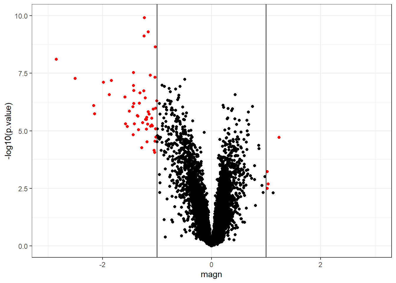
res.de.sim$magn <- magn.sim

A frequently used display is the volcano plot which shows on the y-axis the \(-\log_{10}\) p-values and on the x-axis the magnitude of change. By using \(-\log_{10}\), the “highly significant” features appear at the top of the plot. Using log also permits us to better distinguish between small and very small p-values. We can further highlight the “top genes” as those with adjusted p-value <0.05 and magnitude of change \(>1\).

res.de%>%
  dplyr::mutate(topgene=ifelse(p.value.fdr<0.05&abs(magn)>1,
                               "top",
                               "other")
                )%>%
  ggplot(.,aes(x=magn,y=-log10(p.value),col=topgene))+
  geom_point()+
  scale_color_manual(values = c("top"="red","other"="black"))+
  theme_bw()+
  theme(legend.position = "none")+
  xlim(-3,3)+ylim(0,10)+
  geom_vline(xintercept = 1)+
  geom_vline(xintercept = -1)

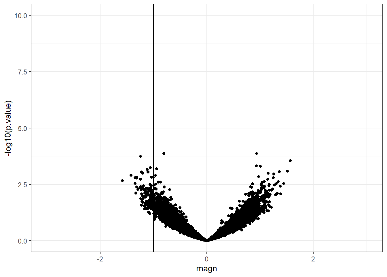
We repeat the same plot with the simulated data.

res.de.sim%>%
  dplyr::mutate(topgene=ifelse(p.value.fdr<0.05&abs(magn)>1,
                               "top",
                               "other")
                )%>%
  ggplot(.,aes(x=magn,y=-log10(p.value),col=topgene))+
  geom_point()+
  scale_color_manual(values = c("top"="red","other"="black"))+
  theme_bw()+
  theme(legend.position = "none")+
  xlim(-3,3)+ylim(0,10)+
  geom_vline(xintercept = 1)+
  geom_vline(xintercept = -1)

7.5 Variance shrinkage and empirical bayes

The basis of the previous analysis is the t-statistic

\[\begin{align*} t_{j}&=\frac{\overline{y}_{j}^B-\overline{y}_{j}^A}{s_{j}\sqrt{\frac{1}{n_A}+\frac{1}{n_B}}}. \end{align*}\]

In a small sample size setting the estimated standard deviations exhibit high variability which can lead to large t-statistics. Extensive statistical methodology has been developed to counteract this challenge. The key idea of those methods is to shrink the gene-wise variances \(\rm s^2_{j}\) towards a common variance \(s^2_0\) (\(s^2_0\) is estimated from the data)

\[\begin{align*} \widetilde{s}_{j}^2&=\frac{d_0 s_0^2+d s^2_{j}}{d_0+d}. \end{align*}\]

A so-called moderated t-statistic is obtained by replacing in the denominator \(s_{j}\) with the “shrunken” \(\widetilde{s}_{j}\). The moderated t-statistic has favourable statistical properties in the small \(n\) setting. The statistical methodology behind the approach is referred to as empirical Bayes and is implemented in the function eBayes of the limma package. Limma starts by running gene-wise linear regression using the lmFit function.

library(limma)

## 
## Attaching package: 'limma'

## The following object is masked from 'package:BiocGenerics':
## 
##     plotMA

# first argument: gene expression matrix with genes in rows and sample in columns
# second argument: design matrix
fit <- lmFit(t(y), design=model.matrix(~ x)) 
head(coef(fit))

##            (Intercept)           xB
## 1367452_at   10.027453  0.092544985
## 1367453_at   10.173732  0.026867630
## 1367454_at   10.275137  0.003017421
## 1367455_at   10.371786 -0.101727288
## 1367456_at   10.815641 -0.006899555
## 1367457_at    9.607297  0.038318498

We can compare it with a standard lm fit.

coef(lm(y[,1]~x)) # gene 1

## (Intercept)          xB 
## 10.02745295  0.09254499

coef(lm(y[,2]~x)) # gene 2

## (Intercept)          xB 
## 10.17373179  0.02686763

Next, the eBayes function is used to calculate the moderated t statistics and p-values.

ebfit <- eBayes(fit)
head(ebfit$t) # moderated t statistics

##            (Intercept)          xB
## 1367452_at    182.4496  1.19066640
## 1367453_at    221.0103  0.41271149
## 1367454_at    184.0507  0.03821825
## 1367455_at    195.0270 -1.35258223
## 1367456_at    257.5965 -0.11619667
## 1367457_at    196.7628  0.55492613

head(ebfit$p.value) # p.values based on moderated t statistics

##             (Intercept)        xB
## 1367452_at 3.871319e-43 0.2441871
## 1367453_at 2.236672e-45 0.6830894
## 1367454_at 3.061059e-43 0.9697959
## 1367455_at 6.452172e-44 0.1874515
## 1367456_at 3.639411e-47 0.9083599
## 1367457_at 5.084786e-44 0.5835310

We can also retrieve the “shrunken” standard deviations

head(sqrt(ebfit$s2.post)) # shrunken standard deviations

## 1367452_at 1367453_at 1367454_at 1367455_at 1367456_at 1367457_at 
##  0.1903875  0.1594624  0.1933930  0.1842254  0.1454464  0.1691410