Chapter 2 The Null Model
2.1 Objective
This exercise uses a mock database for a Happiness Study with undergraduate and graduate students. In this exercise the research question is:
- How happy are the students?
2.2 Load the Data Base
The data base of the Happiness Study is available here. Download the data base load it in the R environment.
Happy <- read.csv("Happy.csv")2.3 Model Estimation
2.3.1 Data Analysis Equation
The fundamental equation for data analysis is data = model + error. In mathematical notation:
\[Y_i=\bar{Y}_i + e_i\]
- \(Y_i\) is the value of the phenomena in subject i;
- \(\bar{Y}_i\) an estimate of the value of the phenomena in subject i;
- \(e_i\) is the diference between the value and the estimated value of the phenomena in subject i.
2.4 The Null Model
The null model is the simplest statistical model for a data set. It is given by a constant estimate:
\[\bar{Y}_i = b_0\]
- \(b_0\) corresponds to the best estimate for our data when there is no independent variable to be modeled.
In the case were the dependent variable is quantitative, \(b_0\) corresponds to the average of the dependent variable:
\[b_0=\bar{X}\]
- \(\bar{X}_i\) corresponds to the average of the dependent variable.
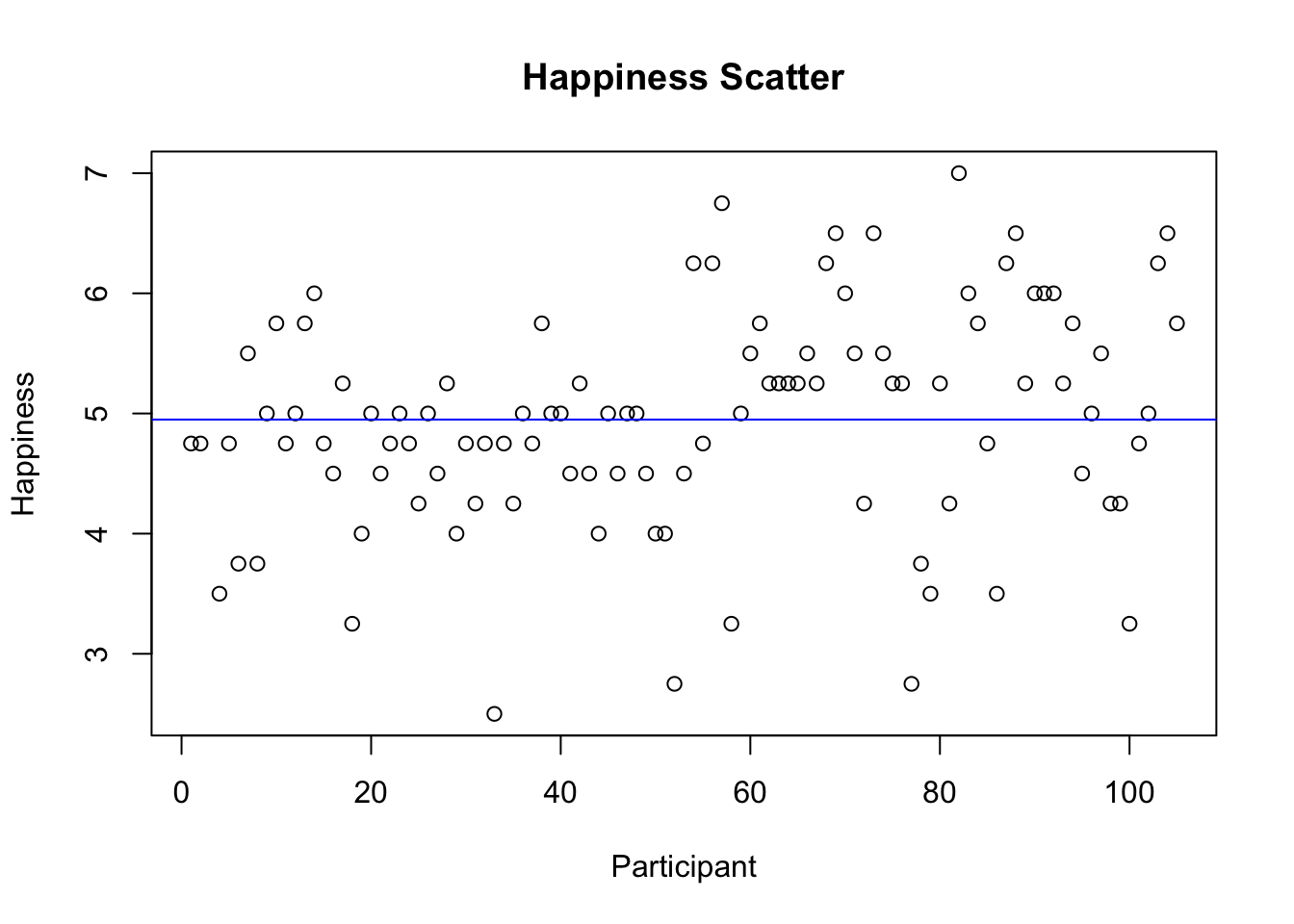
Represent the null model:
- Using the
summaryfunction and record the mean value; - Plotting the average in a scatter with the functions
plotandabline; - Create a constant in the database with the mean value and look at the data frame with the
headfunction.
summary(Happy$HappyScale) # Descriptives## Min. 1st Qu. Median Mean 3rd Qu. Max.
## 2.50 4.50 5.00 4.95 5.50 7.00plot(Happy$ID, Happy$HappyScale, type = 'p',
ylab = 'Happiness', xlab = 'Participant', main='Happiness Scatter') # Scatter
abline(h=(mean(Happy$HappyScale)), col="blue") # Plot constant in the scatter
Happy$nullmodel <- mean(Happy$HappyScale) # Represent estimate of the null model in the database
head(Happy, n=5)
## ID Age Edu Gender HappyScale EmotinalSup InstruSup Popularity Wealth
## 1 1 23 17 1 4.75 4.00 4 5 6
## 2 2 26 16 1 4.75 3.25 4 2 3
## 3 4 23 17 0 3.50 3.00 3 5 4
## 4 5 23 17 0 4.75 4.00 4 3 7
## 5 6 24 17 1 3.75 4.00 4 4 4
## nullmodel
## 1 4.949519
## 2 4.949519
## 3 4.949519
## 4 4.949519
## 5 4.9495192.4.1 The Null Model Error
Models are estimates, simplifications of the data we observed. Consequently, every model has error. The error is given by the difference between the data and the model:
\[e_i=Y_i-\bar{Y}_i\]
Represent the null model error:
- Represent the difference between the data (\(Y_i\)) and the model (\(\bar{Y}_i\)) in the database.
Happy$nullmodelerror <- Happy$HappyScale-Happy$nullmodel # difference between the data and model
head(Happy, n=5)
## ID Age Edu Gender HappyScale EmotinalSup InstruSup Popularity Wealth
## 1 1 23 17 1 4.75 4.00 4 5 6
## 2 2 26 16 1 4.75 3.25 4 2 3
## 3 4 23 17 0 3.50 3.00 3 5 4
## 4 5 23 17 0 4.75 4.00 4 3 7
## 5 6 24 17 1 3.75 4.00 4 4 4
## nullmodel nullmodelerror
## 1 4.949519 -0.1995192
## 2 4.949519 -0.1995192
## 3 4.949519 -1.4495192
## 4 4.949519 -0.1995192
## 5 4.949519 -1.1995192The most intuitive solution to calculate the total error of a model is to add the error for each single case. However, this solution has a problem - the errors would cancel out because they have different signs.The statistical solution to calculate the total error of a model to perform the sum of square errors (SSE). Squaring the errors ensures that i) errors do not cancel out when added together and that ii) errors have weighted weights where larger errors weigh more than smaller errors (e.g., four errors of 1 squared and added together are worth 4 while that 3 errors of 0 and 1 error of 4 squared and added together are worth 16). The SSE is the conventional measure of error used in statistics to measure the performance of statistical models.
Represent the null model squared error:
- Represent the squared difference between the data (\(Y_i\)) and the model (\(\bar{Y}_i\)) in the database;
- Compute the sum of the errors and of the sum of the squared erros (SSE) using the
sumfunction.
Happy$nullmodelerroSQR <- (Happy$HappyScale-Happy$nullmodel)^2 # squared difference between the data and model
sum(Happy$nullmodelerror) # sum of the errors
## [1] -0.000000000000007105427sum(Happy$nullmodelerroSQR) # sum of the squared errors## [1] 84.92248head(Happy, n=5)## ID Age Edu Gender HappyScale EmotinalSup InstruSup Popularity Wealth
## 1 1 23 17 1 4.75 4.00 4 5 6
## 2 2 26 16 1 4.75 3.25 4 2 3
## 3 4 23 17 0 3.50 3.00 3 5 4
## 4 5 23 17 0 4.75 4.00 4 3 7
## 5 6 24 17 1 3.75 4.00 4 4 4
## nullmodel nullmodelerror nullmodelerroSQR
## 1 4.949519 -0.1995192 0.03980792
## 2 4.949519 -0.1995192 0.03980792
## 3 4.949519 -1.4495192 2.10110600
## 4 4.949519 -0.1995192 0.03980792
## 5 4.949519 -1.1995192 1.43884638The SEQ indicates that the average happiness of 4.9495192 has an error of 84.922476 total square happiness. Note that the error in total square happiness is a problem because:
- it is a total (the more observations, the more error);
- it is squared (does not allow a direct comparison with the original measure).
Considering that the SSE is:
\[SSE=\displaystyle\sum\limits_{i=1}^n e_i^2\]
The average of the SSE is the variance and can be computed using:
\[s^2=\frac{SSE}{n-p}\]
The square root of the SSE is the standard-deviation and can be computed using:
\[s=\sqrt{s^2}\]
Compute the SSE, variance and standard-deviation using the formulas above and running the functions var and sd.
var_y <- sum(Happy$nullmodelerroSQR)/(length(Happy$HappyScale)-1) # variance
sd_y <- sqrt(var_y) # standard deviation
var_y # print the variance computed by hand
## [1] 0.8244901var(Happy$HappyScale) # compare## [1] 0.8244901sd_y # print the standard deviation computed by hand ## [1] 0.9080143sd(Happy$HappyScale) # compare## [1] 0.90801432.4.2 The Fundamental Principle of Data Analysis
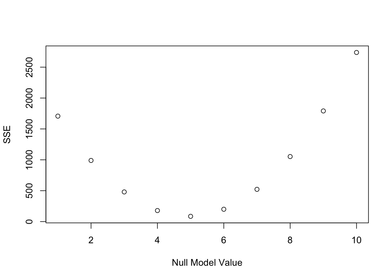
The fundamental principle of data analysis is to minimize the error associated with a model. The lower the model error, the closer the model is to the data, and the better the model is. Error minimization is done using the Ordinary Squares Method (OLS). According to the OLS, the average is the best model to represent our data in a model without a VI and with a metric DV!
See bellow the SSE for possibles values of the null model. As expected, the model with lower SSE is the one with 4.9495192.

2.4.3 Model Estimation Conclusion
The null model and null model error show that:
- the mean happiness of the students is:
mean(Happy$HappyScale) ## [1] 4.949519- the average error associated with the mean is:
sd(Happy$HappyScale) ## [1] 0.90801432.5 The Experienced Researcher
Experienced Researchers report promptly the results of the model estimation, they don’t need to estimate in detail the null model and the error of the null mode. The calculation of the null model and error of the null model is a demonstration of the origin and meaning of these concepts (model and error) in the context of the simplest type of research problem possible.
- Why do we need models? Our data are usually bulky and of a form that is hard to communicate to others. The compact description provided by the models is much easier to communicate.
- How do we know which model is best? The minimization of error in linear models is done according to the Ordinary Least Squares Method (OLS). According to this method, when we have only one DV, the best null model is: for a metric DV, the average; for an ordinal RV, the median; and for a nominal DV, the mode.
- Why do we need a model as simple as the null model? The null model is the model against which we can compare the performance of more complex models that model the effects of IVs in a DV. A more complex model is only better than a null model if it manages to have less error than the null model!
- When do we look at models with VIs? The next classes are dedicated entirely to modeling the effects of IVs in a DV. For now, keep in mind the data analysis equation and the concepts of null model and null model error.
- Why don’t we talk about measures of central tendency or descriptive statistics? Averages, modes and medians are often referred to as measures of central tendency. Here we treat these measures as models, simplifications of our data.
- And why don’t we talk about dispersion measures? Sum of square errors, variance, standard deviation and standard error are often referred to as data dispersion measures. Here we treat these dispersion measures as error measures, the deviation between data and model.
2.6 Knowledge Assessment
Here is what you should know by now:
- What is the basic equation for data analysis?
- What is the null model?
- What are the most famous (null) models?
- What is the error associated with the null model?
- How is the error of a model measured?
- What is the fundamental principle of data analysis?