Chapter 4 Multiple Linear Model

4.1 Objective

This exercise uses a mock database for a Happiness Study with undergraduate and graduate students. In this exercise the research question is:

Does self-perceptions, namely, perceived popularity and wealth, influence the level o happiness of students;
Another way to make the same questions could be: what is the relation between self-perceptions and heath.

In this case we have specific prediction, we expect that higher self-perceptions to be associated with higher levels of happiness.

4.2 Load the Data Base

The data base of the Happiness Study is available here. Download the data base load it in the R environment.

Happy <- read.csv("Happy.csv")

4.3 Model Estimation

4.3.1 Data Analysis Equation

In review, The fundamental equation for data analysis is data = model + error. In mathematical notation:

\[Y_i=\bar{Y}_i + e_i\]

$Y_i$ is the value of the phenomena in subject i;
$\bar{Y}_i$ an estimate of the value of the phenomena in subject i;
$e_i$ is the difference between the value and the estimated value of the phenomena in subject i.

4.3.2 The Proposed Model

In review, the proposed model is a more complete statistical model for our data. This model makes specific predictions for every observation base on one or more independent variables of interest (IV). The notation for this model is:

\[\bar{Y}_i = b_0+b_1\times X_{i1}...b_j\times X_{ij}\]

$b_0$ corresponds to?the best estimate for our data when the independent variables are 0;
$b_1$ is the parameter estimating the effect of the independent variable $1$ for every subject $i$;
$b_j$ is the $j$ parameter estimating the effect of the IV $j$ for every subject $i$.

In the case of our research problem (i.e., does perceived popularity and wealth, influence the level o happiness of students?) the proposed model is:

\[\bar{Happiness}_i = b_0+b_1\times{popularity_{i}}+b_2\times{wealth_{i}}\]

$b_0$ correspondes to the best estimate for the level of happiness when the independent variable $Age$ is $0$ for the subject $i$;
$b_1$ is the parameter estimating the effect of $popularity$ on subject $i$;
$b_2$ is the parameter estimating the effect of $wealth$ on subject $i$.

Note that we could calculate the parameters of the proposed model by had using the appropriate formulas. Here we follow a simpler approach and ask R to compute the parameters of the model for us.

Compute the parameters for the proposed model using the lm() function and represent the model in a 3 dimensional graph using the scatterplot3d() functions.

Model.2 <- lm(Happy$HappyScale~Happy$Popularity+Happy$Wealth)
summary(Model.2)

## 
## Call:
## lm(formula = Happy$HappyScale ~ Happy$Popularity + Happy$Wealth)
## 
## Residuals:
##      Min       1Q   Median       3Q      Max 
## -2.48040 -0.48951 -0.04461  0.50625  2.24289 
## 
## Coefficients:
##                  Estimate Std. Error t value          Pr(>|t|)    
## (Intercept)       4.00748    0.42689   9.388 0.000000000000002 ***
## Happy$Popularity  0.14790    0.07850   1.884            0.0624 .  
## Happy$Wealth      0.05591    0.07649   0.731            0.4665    
## ---
## Signif. codes:  0 '***' 0.001 '**' 0.01 '*' 0.05 '.' 0.1 ' ' 1
## 
## Residual standard error: 0.8923 on 101 degrees of freedom
## Multiple R-squared:  0.05302,    Adjusted R-squared:  0.03427 
## F-statistic: 2.827 on 2 and 101 DF,  p-value: 0.06386

library(scatterplot3d) # function scatterplot3d
Model.2.plot <- scatterplot3d(
  x=Happy$Popularity, 
  y=Happy$Wealth, 
  z=Happy$HappyScale, type="p") # 3d plot of our model
Model.2.plot$plane3d(Model.2, draw_polygon = TRUE, draw_lines = TRUE)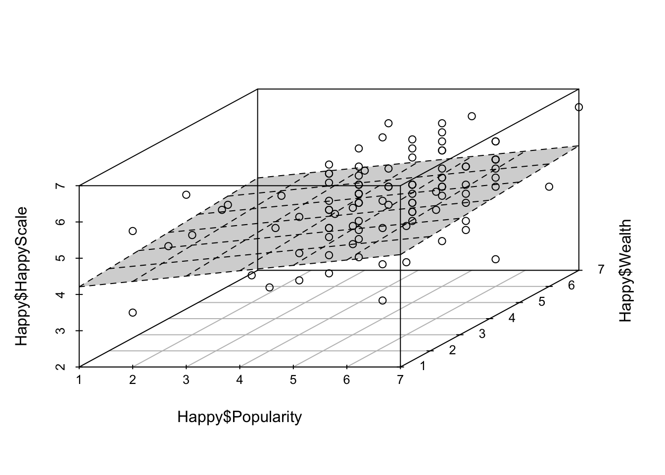

Based on the output, the equation for the proposed model can be written like this using the extract_eq()function:

library(equatiomatic)
extract_eq(Model.2)

\[ \operatorname{Happy\$HappyScale} = \alpha + \beta_{1}(\operatorname{Happy\$Popularity}) + \beta_{2}(\operatorname{Happy\$Wealth}) + \epsilon \]

With this equation compute the proposed model estimates for every subject and corresponding error.

Happy$propmodel <- 4.00748+0.14790*Happy$Popularity+0.05591*Happy$Wealth  # proposed model
Happy$propmodelerroSQR <- (Happy$HappyScale-Happy$propmodel)^2 # squared difference
sum(Happy$propmodelerroSQR) # sum of the squared erros of the proposed model

## [1] 80.42002

The total error for our proposed model is 80.4200231.

4.3.3 Model Comparison

To address our research question, we can say that the self-perceptions have an effect on happiness only if the proposed model $\bar{Happiness}_i = b_0+b_1\times{popularity_{i}}+b_2\times{wealth_{i}}$ has less error that the null model $\bar{Happiness}_i = b_0$. In other words, if the proposed model has less error that the null model we can say that at least one of the the parameters, $b_1$ estimating the effect of popularity and or $b_2$ estaimaitng the effect of wealth, reduces the estimation error of the null model with the constant $b_0$.

To compare the proposed and null model we first need to compute the SSE of the null model:

Happy$nullmodel <- mean(Happy$HappyScale) # null model
Happy$nullmodelerroSQR <- (Happy$HappyScale-Happy$nullmodel)^2 # squared difference
sum(Happy$nullmodelerroSQR) # sum of the squared erros of the null model

## [1] 84.92248

The total error for our null model is 84.922476.

To compare the null model and the proposed model compute the proportion of the reduction of the error (PRE) according to equation:

\[PRE=\frac{SSE_{null}-SSE_{proposed}}{SSE_{null}}\]

Model.2.PRE <- (sum(Happy$nullmodelerroSQR)-sum(Happy$propmodelerroSQR))/sum(Happy$nullmodelerroSQR)
Model.2.PRE

## [1] 0.05301839

The Proportion of the Reduction of Error (PRE) in this case is 0.0530184. This indicates that the Proposed Model reduces the error of the Null Model in $5.3\%$.

To compare the null model and the proposed model in R you can use the aov(), anova() and summary(lm())functions. Compute these functions as indicated below.

aov(Model.2) # SSE details

## Call:
##    aov(formula = Model.2)
## 
## Terms:
##                 Happy$Popularity Happy$Wealth Residuals
## Sum of Squares           4.07697      0.42548  80.42002
## Deg. of Freedom                1            1       101
## 
## Residual standard error: 0.8923216
## Estimated effects may be unbalanced

anova(Model.2) # even more SSE details

## Analysis of Variance Table
## 
## Response: Happy$HappyScale
##                   Df Sum Sq Mean Sq F value  Pr(>F)  
## Happy$Popularity   1  4.077  4.0770  5.1203 0.02579 *
## Happy$Wealth       1  0.425  0.4255  0.5344 0.46647  
## Residuals        101 80.420  0.7962                  
## ---
## Signif. codes:  0 '***' 0.001 '**' 0.01 '*' 0.05 '.' 0.1 ' ' 1

summary(lm(Model.2)) # PRE value

## 
## Call:
## lm(formula = Model.2)
## 
## Residuals:
##      Min       1Q   Median       3Q      Max 
## -2.48040 -0.48951 -0.04461  0.50625  2.24289 
## 
## Coefficients:
##                  Estimate Std. Error t value          Pr(>|t|)    
## (Intercept)       4.00748    0.42689   9.388 0.000000000000002 ***
## Happy$Popularity  0.14790    0.07850   1.884            0.0624 .  
## Happy$Wealth      0.05591    0.07649   0.731            0.4665    
## ---
## Signif. codes:  0 '***' 0.001 '**' 0.01 '*' 0.05 '.' 0.1 ' ' 1
## 
## Residual standard error: 0.8923 on 101 degrees of freedom
## Multiple R-squared:  0.05302,    Adjusted R-squared:  0.03427 
## F-statistic: 2.827 on 2 and 101 DF,  p-value: 0.06386

4.4 Statistical Inference

Here we will run the appropriate statistical test and look for the corresponding test statistics and p-value on the output. For more details about the basic concepts in Statistical Inference see 3.4.1.

4.4.1 Model Overview

At this point we know that:

$b_1=0.15$, meaning that Popularity has a positive association with Happiness;
$b_2=0.06$, meaning that Wealth has also a positive (but almost null) assocaition with Happiness;
$PRE=0.05$, meaning that the proposed model with Popularity and Wealth support is 5% better than the null model.

Statistical inference is method that allows to determine if the estimates produced for our sample (i.e., $b_1$, $b_2$, and $PRE$) can be generalized to the the population where the data was collected. In other words, it is the method to test the likelihood of an estimate for our sample to happen by chance if the value is generalized to the population. In our case, this means:

How likely is the value of $b_1=0.15$ in our sample to result form chance?
How likely is the value of $b_2=0.06$ in our sample to result form chance?
How likely is the difference in error of 5% between the null and the proposed model in our sample to result from chance?

4.4.2 Inference for $PRE$

The statistical inference for $PRE$ tests the likelihood of the reduction of the error of the proposed model relative to the the null model observed in the sample (the $R^2$ value) happening by chance if the value is generalized to the population.

The statistical hypothesis for this inference is given by the following notation:

\[H_0:\eta^2=0\;vs\;H_1:\eta^2\neq0\]

$H_0$ corresponds to the null hypothesis and states that the the reduction of the error of the proposed model observed is the sample ($R^2$) is likely to have happened by chance if the value is generalized to the population ($\eta^2$).
$H_1$ corresponds to the alternative hypothesis and states that the the reduction of the error of the proposed model observed is the sample ($R^2$) is not likely to have happened by chance if the value is generalized to the population ($\eta^2$).

The value of the test statistic and the corresponding p-value for this inference is $F=2.83$ and $p-value=0.06$. Considering that $p-value\leq0.05$, the test statistics is likely to have happened by chance. Consequently, the decision for this test is not to reject $H_0$, meaning that the reduction of the error of the proposed model relative to the the null model observed in the sample is not statistically significant.

4.4.3 Inference for $b_1$

The statistical inference for $b_1$ tests the likelihood of the assocaition between Popularity and Happiness in the sample (represented by $b_1$) happening by chance if the value of this effect is generalised to the population.

The statistical hypothesis for this inference is given by the following notation:

\[H_0:\beta_1=0\;vs\;H_1:\beta_1>0\]

$H_0$ corresponds to the null hypothesis and states that the effect of Popularity ($b_1$) is likely to have happened by chance if the value is generalised to the population ($\beta_1$);
$H_1$ corresponds to the alternative hypothesis and states that a positive effect of Popularity ($b_1$) is not likely to have happened by chance if the value is generalised to the population ($\beta_1$).

The value of the test statistic and the corresponding p-value for this inference is $t=1.88$ and $p-value=\frac{0.06}{2}$. Considering that $p-value\leq0.05$, the test statistics has a high likelihood of happening by chance. Consequently, the decision for this test is to reject $H_0$, meaning that that the effect of Popularity observed in the sample is statistically significant.

Note that the $p-value=\frac{0.06}{2}$ (and not $p-value=0.06$) because we have a unilateral hypothesis testing with a $H_1:\beta_1>0$. Here we are interested in the likelihood of getting a test statistic that is equal or higher $Pr(>t)$ (and not equal or more extreme $Pr(>|t|)$)!

4.4.4 Inference for $b_2$

The statistical inference for $b_2$ tests the likelihood of the correlation between Wealth and Happiness in the sample (represented by $b_2$) happening by chance if the value of this effect is generalised to the population.

The statistical hypothesis for this inference is given by the following notation:

\[H_0:\beta_2=0\;vs\;H_1:\beta_2>0\]

$H_0$ corresponds to the null hypothesis and states that the effect of Wealth ($b_2$) is likely to have happened by chance if the value is generalised to the population ($\beta_2$).
$H_1$ corresponds to the alternative hypothesis and states that a positive effect of Wealth ($b_2$) is not likely to have happened by chance if the value is generalised to the population ($\beta_2$).

The value of the test statistic and the corresponding p-value for this inference is $t=-0.41$ and $p-value=1-\frac{0.63}{2}$ (again, a uniletral testing!). Considering that $p-value>0.05$, the test statistics has a high likelihood of happening by chance. Consequently, the decision for this test is to reject $H_0$, meaning that that the effect of Wealth observed in the sample is not statistically significant.

4.5 Model Estimation and Statistical Inference Conclusion

Remember that experienced researchers report promptly the results of the model estimation, they don’t need to estimate in detail the null a proposed models nor the hypothesis testing process. These serve as a demonstration of the origin and meaning of the concepts of model, error, effect, test statistic and p-value in the context of the simplest type of proposed model. Here is an example of how to write down the results.

With this analysis we want to study the role of two elements of self-perception, popularity and wealth, on happiness. The results indicate that the model with popularity and wealth reduces the error of the null model by approximately 5% and that this effect is marginally significant with F=2.83 p = 0.06. The analysis of the betas indicates that the magnitude of the association of both popularity and wealth with happiness is weak, respectively, beta=0.19 and beta=0.08, but still the association of popularity is stringer and reaches statistical significance, respectively, t=1.88, p=0.03 (unilateral) and t=0.73, p=0.24 (unilateral).

4.5.1 Parameters ($b_s$) and Standerdized Parameters ($betas_s$)

Multiple linear regressions impose an additional constrain for interpretation. In the case of this exercise, the three parameters in the proposed model equation ($b_0$, $b_1$, and $b_3$) have a tridimensional representation. This representation makes the parameters ($b$ values) difficult to interpret. Consequently, in multiple linear regressions the parameters are converted into standardised parameters ($beta$ values). Standardised parameters are also known as correlations and they can vary between -1 and 1, despite of the way the variables in consideration were originally measured. Correlations give a sense of the magnitude (or strength) of association between variables, with more extreme values (i.e., closer to -1 or 1) being indicative of stronger the correlations. A qualitative interpretation of the magnitudes that is the convention is Social Sciences is depicted in the figure bellow (for more details, see Hemphill, 2003¹).

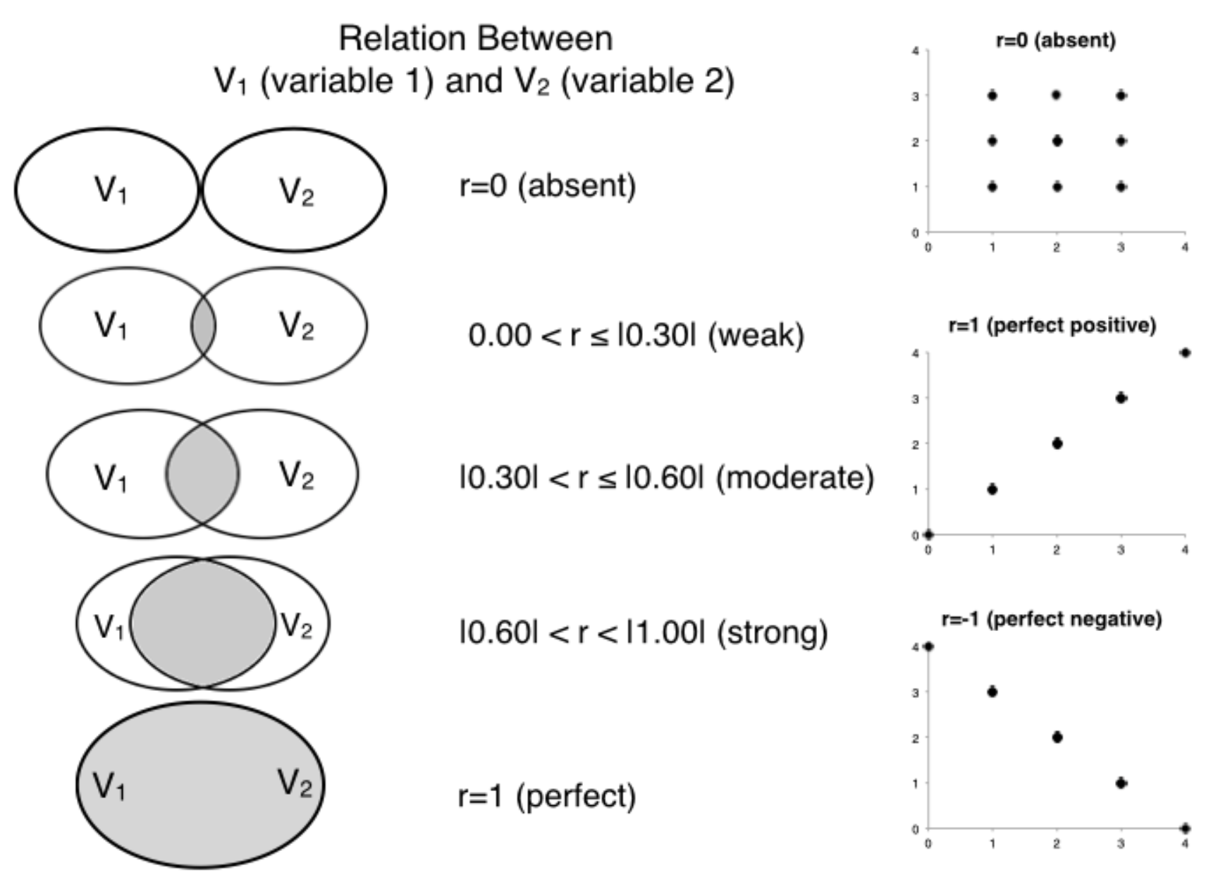
Magnitudes of correlation between two variables.

Compute the standardised parameters for the proposed model using the lm.beta() function (requires the lm.beta package).

library(lm.beta) # lm.beta function
summary(lm.beta(Model.2 ))

## 
## Call:
## lm(formula = Happy$HappyScale ~ Happy$Popularity + Happy$Wealth)
## 
## Residuals:
##      Min       1Q   Median       3Q      Max 
## -2.48040 -0.48951 -0.04461  0.50625  2.24289 
## 
## Coefficients:
##                  Estimate Standardized Std. Error t value          Pr(>|t|)    
## (Intercept)       4.00748      0.00000    0.42689   9.388 0.000000000000002 ***
## Happy$Popularity  0.14790      0.19377    0.07850   1.884            0.0624 .  
## Happy$Wealth      0.05591      0.07518    0.07649   0.731            0.4665    
## ---
## Signif. codes:  0 '***' 0.001 '**' 0.01 '*' 0.05 '.' 0.1 ' ' 1
## 
## Residual standard error: 0.8923 on 101 degrees of freedom
## Multiple R-squared:  0.05302,    Adjusted R-squared:  0.03427 
## F-statistic: 2.827 on 2 and 101 DF,  p-value: 0.06386

Based on this output we can say that both Popularity and Wealth have week correlations correlations Happiness, respectively $beta_1=0.19$ and $beta_2=0.08$, although the effect of Popularity is twice as big as that of Wealth.

4.5.2 Standerdized Parameters ($betas_s$) as partial correlations

$Betas$ not only are important because they represent the association between two variables in a standardized measure - $betas$ also control for the specific effect of each IV. In other words, the $betas$ in a multiple linear regression estimate partial correlations representing the amount of unique variance accounted by each independent variable $X_1$ (e.g., Popularity) relative to the variance of the dependent variable $Z$ (i.e., Happiness) that can not not be accounted the other independent variables $X_i$ (e.g., Wealth).

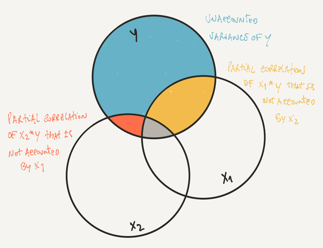
Schematic representation of a partial correlation of $X1$ controlling for the effect of $X2$.

Run the bivariate correaltions between each IV and the DV and compare with the the standardised parameters in the regression above - diferent right? That is because the $betas$ are similar to bivariate correlations (in the way you interpret them) but not exactly the same (because they account fot the effect of other IVs in the model!).

cor(Happy$HappyScale, Happy$Popularity)

## [1] 0.2191076

cor(Happy$HappyScale, Happy$Wealth)

## [1] 0.1404823

4.5.3 Model estimation and statistical inference revisited

With this analysis we want to study the role of two elements of self-perception, popularity and wealth, on happiness.The results indicate that the model with popularity and wealth reduces the error of the null model by approximately 5%. The analysis of the estimated parameters indicates that the greater the popularity and wealth the greater the happiness, respectively b=0.15 and b=0.06. The betas analysis indicates that the magnitude of the association of both popularity and wealth with happiness is weak (respectively, beta=0.19 and beta=0.08) but still the association of popularity is is a more important predictor than wealth.

4.6 More About… interpreting effects in linear modeling

4.6.1 Is there an order to report statisitical inference?

The statistical inference of the estimates of a model always starts with the inference for $PRE$ because this is an estimate for the general performance of the model. After follows the inference for $b_s$, the estimates for the specific performance of the parameters modelling the effects of the independent variables. In the case of models with only one independent variable, the statistical inference for $PRE$ is redundant with the statistical inference for $b_1$ because all the reduction of the error results from the effect of this independent variable. But with models with two or more parameters $PRE$ is crucial to evaluate the model performance.

4.6.2 What exaclty is a unilateral hypotesis testing?

The hypothesis testing for both $b_1$ and $b_2$ is a unilateral hypothesis testing. This means that we interested in testing the likelihood of $\beta_1>0$ and $\beta_2>0$ (an not the bilateral option of $\beta_1\neq0$ and $\beta_2\neq0$). To understand the unilateral hypothesis testing is its crucial to keep in mind that the statistical test is blind to our hypothesis - the $p-value$ given for each parameter simply corresponds to the likelihood the corresponding test statistics to be equal of more extreme. Consequently, the likelihood of the test statistics to the be equal of higher to the tests statistics needs additional computations: i) often, this simply means to divid the $p-value$ in half; however, ii) in cases where the test statistics has a different value of the one predicted (e.g., the $test\;statistics<0$ but the hypothesis was that the $\beta>0$) this means do divide the $1-p-value$ (the inverse $p-value$) in half. See the figures bellow with the illustration of the unilateral hypothesis testing for $\beta_1>0$ and $\beta_2>0$.

Hemphill, J. F. (2003). Interpreting the magnitudes of correlation coefficients. The American Psychologist, 58(1), 78?79. https://doi.org/10.1037/0003-066X.58.1.78 ↩︎

Step by Step I: Linear Models

Chapter 4 Multiple Linear Model

4.1 Objective

4.2 Load the Data Base

4.3 Model Estimation

4.3.1 Data Analysis Equation

4.3.2 The Proposed Model

4.3.3 Model Comparison

4.4 Statistical Inference

4.4.1 Model Overview

4.4.2 Inference for \(PRE\)

4.4.3 Inference for \(b_1\)

4.4.4 Inference for \(b_2\)

4.5 Model Estimation and Statistical Inference Conclusion

4.5.1 Parameters (\(b_s\)) and Standerdized Parameters (\(betas_s\))

4.5.2 Standerdized Parameters (\(betas_s\)) as partial correlations

4.5.3 Model estimation and statistical inference revisited

4.6 More About… interpreting effects in linear modeling

4.6.1 Is there an order to report statisitical inference?

4.6.2 What exaclty is a unilateral hypotesis testing?