Chapter 3 Simple Lineal Model

3.1 Objective

This exercise uses a mock database for a Happiness Study with undergraduate and graduate students. In this exercise the research question is:

Does age predicts the level of happiness among students?
Another way to make this same question could be: are age and happiness correlated?

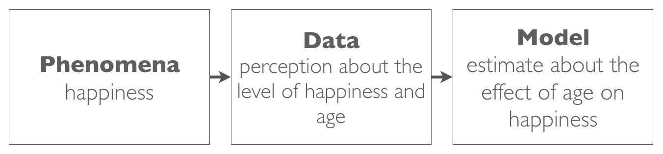
Schematic representation of the research question.

3.2 Load the Data Base

The data base of the Happiness Study is available here. Download the data base load it in the R environment.

Happy <- read.csv("Happy.csv")

3.3 Model Estimation

3.3.1 Data Analysis Equation

In review, The fundamental equation for data analysis is data = model + error. In mathematical notation:

\[Y_i=\bar{Y}_i + e_i\]

$Y_i$ is the value of the phenomena in subject i;
$\bar{Y}_i$ an estimate of the value of the phenomena in subject i;
$e_i$ is the difference between the value and the estimated value of the phenomena in subject i.

3.3.2 The Proposed Model

The proposed model is a more complete statistical model for our data. This model makes specific predictions for every observation base on one or more independent variables of interest (IV). The notation for this model is:

\[\bar{Y}_i = b_0+b_1X_{i1}...b_jX_{ij}\]

$b_0$ corresponds to?the best estimate for our data when the independent variables are 0;
$b_1$ is the parameter estimating the effect of the independent variable $1$ for every subject $i$;
$b_j$ is the $j$ parameter estimating the effect of the IV $j$ for every subject $i$.

In the case of our research problem (i.e., does age predict the level of happiness?) the proposed model is:

\[\bar{Happiness}_i = b_0+b_1age_{i}\]

$b_0$ corresponds to the best estimate for the level of happiness when the independent variable $Age$ is $0$ for the subject $i$;
$b_1$ is the parameter estimating the effect of $Age$ on subject $i$.

3.3.2.1 Model Estimation By Hand

For a Model I we could calculate the full model parameters with the following formulas:

\[b_0=\bar{Y}-b_1\bar{X}\]

$\bar{Y}$ is the mean of the dependent variable;
$\bar{Y}$ is the mean of the independent variable.

$b_1$ is given by:

\[b_1=\frac{Cov_{xy}}{s^2_X}\]
- $s^2_X$ is the variance of the independent variable; - $Cov_{xy}$ is the covariance between the independent variable and the dependent variable and is given by:

\[Cov_{xy}=\frac{SPE}{N-p}\]

$SPE$ is the sum of product of errors of the independent variable and dependent variable;
$N$ is sample size;
$p$ is the number of parameters used to calculate the $SPE$.

Here we follow a simpler approach and ask R to compute the parameters of the model for us.

3.3.2.2 Model Estimation in a Simple Linear Regression

Compute the parameters for the proposed model using the lm() function and represent the model in a graph using the plot() and abline() functions.

Model.1 <- lm(Happy$HappyScale~Happy$Age)
summary(Model.1)

## 
## Call:
## lm(formula = Happy$HappyScale ~ Happy$Age)
## 
## Residuals:
##      Min       1Q   Median       3Q      Max 
## -2.50321 -0.45605  0.04395  0.55338  1.95907 
## 
## Coefficients:
##             Estimate Std. Error t value            Pr(>|t|)    
## (Intercept)  5.41819    0.44337  12.220 <0.0000000000000002 ***
## Happy$Age   -0.01886    0.01748  -1.079               0.283    
## ---
## Signif. codes:  0 '***' 0.001 '**' 0.01 '*' 0.05 '.' 0.1 ' ' 1
## 
## Residual standard error: 0.9073 on 102 degrees of freedom
## Multiple R-squared:  0.01129,    Adjusted R-squared:  0.001592 
## F-statistic: 1.164 on 1 and 102 DF,  p-value: 0.2831

plot(Happy$Age, Happy$HappyScale, 
     xlab="Age", 
     ylab="Happiness", 
     main="Scatter Age by Happiness")
abline(lm(Happy$HappyScale~Happy$Age), col="blue")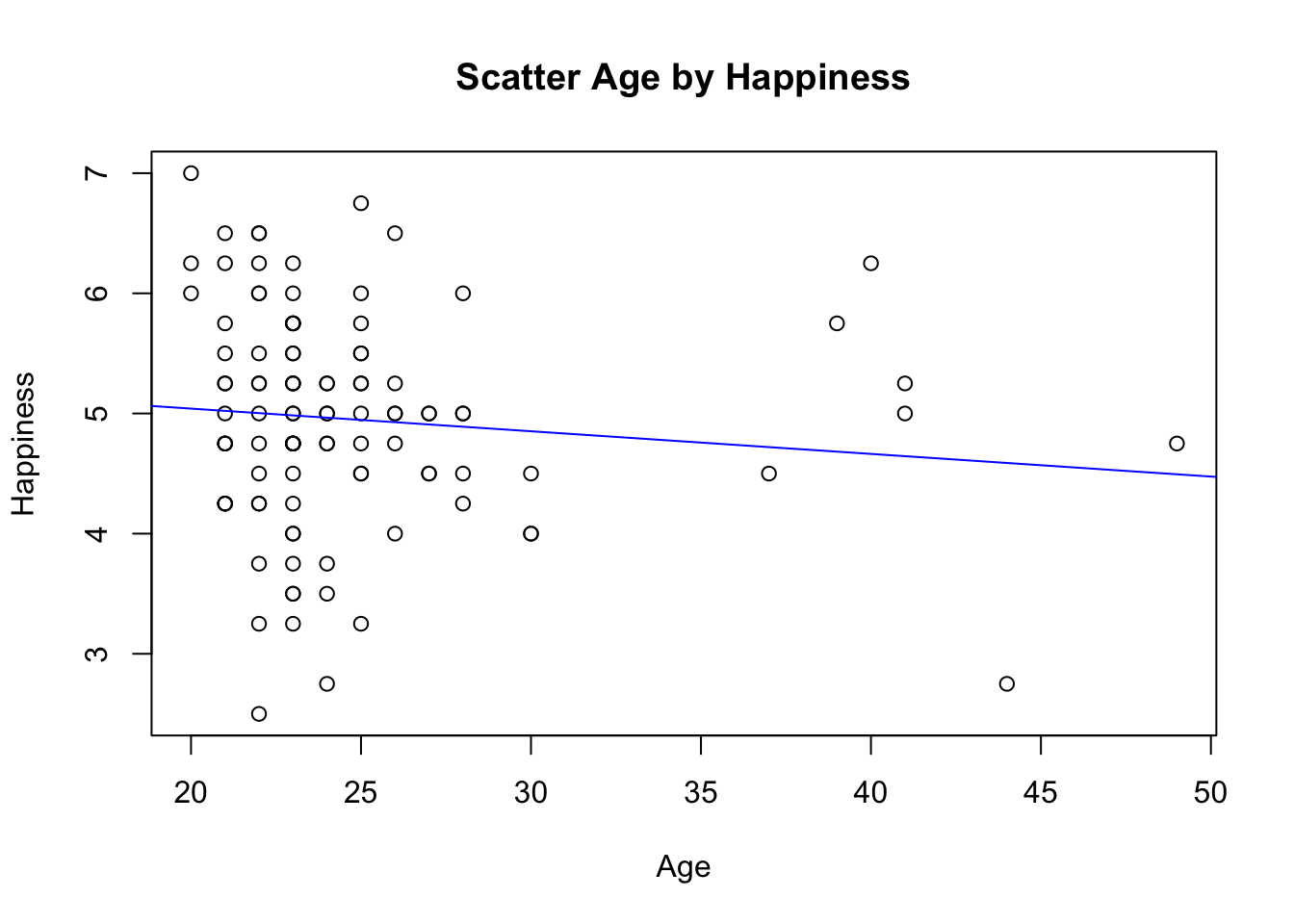

Based on the output, the equation for the proposed model can be written like this using the extract_eq()function:

extract_eq(Model.1)

\[ \operatorname{Happy\$HappyScale} = \alpha + \beta_{1}(\operatorname{Happy\$Age}) + \epsilon \]

With this equation compute the proposed model estimates for every subject and corresponding error.

# Proposed Model
Happy$propmodel <- 5.41819-0.01886*Happy$Age
# Proposed Model Error
Happy$propmodelerroSQR <- (Happy$HappyScale-Happy$propmodel)^2
sum(Happy$propmodelerroSQR)

## [1] 83.9641

The total error for our proposed model is 83.9641009.

3.3.3 Model Comparisson

To address our research question, we can say age has an effect on happiness only if the proposed model $\bar{Happiness}_i = b_0+b_1age_{i}$ has less error that the null model $\bar{Happiness}_i = b_0$. In other words, if the proposed model has less error that the null model we can say that the parameter $b_1$ estimating the effect of age on happiness reduces the error in the data and contributes to a better model than the null model with the constant $b_0$

To compare the proposed and null model we first need to compute the SSE of the null model:

# Null Model
Happy$nullmodel <- mean(Happy$HappyScale)
# Null Model Error
Happy$nullmodelerroSQR <- 
  (Happy$HappyScale-Happy$nullmodel)^2
sum(Happy$nullmodelerroSQR)

## [1] 84.92248

The total error for our null model is 84.922476.

To compare the null model and the proposed model compute the proportion of the reduction of the error (PRE) according to equation:

\[PRE=\frac{SSE_{null}-SSE_{proposed}}{SSE_{null}}\]

Model.I.PRE <- (sum(Happy$nullmodelerroSQR)-sum(Happy$propmodelerroSQR))/sum(Happy$nullmodelerroSQR)
Model.I.PRE

## [1] 0.01128529

The Proportion of the Reduction of Error (PRE) in this case is 0.0112853. This indicates that the Proposed Model reduces the error of the Null Model in $1.1\%$.

To compare the null model and the proposed model in R you can use the aov() and summary(lm())functions. Compute these functions as indicated bellow.

aov(Model.1) # SSE details

## Call:
##    aov(formula = Model.1)
## 
## Terms:
##                 Happy$Age Residuals
## Sum of Squares    0.95838  83.96410
## Deg. of Freedom         1       102
## 
## Residual standard error: 0.9072913
## Estimated effects may be unbalanced

summary(lm(Model.1)) # PRE value

## 
## Call:
## lm(formula = Model.1)
## 
## Residuals:
##      Min       1Q   Median       3Q      Max 
## -2.50321 -0.45605  0.04395  0.55338  1.95907 
## 
## Coefficients:
##             Estimate Std. Error t value            Pr(>|t|)    
## (Intercept)  5.41819    0.44337  12.220 <0.0000000000000002 ***
## Happy$Age   -0.01886    0.01748  -1.079               0.283    
## ---
## Signif. codes:  0 '***' 0.001 '**' 0.01 '*' 0.05 '.' 0.1 ' ' 1
## 
## Residual standard error: 0.9073 on 102 degrees of freedom
## Multiple R-squared:  0.01129,    Adjusted R-squared:  0.001592 
## F-statistic: 1.164 on 1 and 102 DF,  p-value: 0.2831

plot(Happy$Age, Happy$HappyScale, 
     xlab="Age", 
     ylab="Happiness", 
     main="Scatter Age by Happiness")
abline(lm(Happy$HappyScale~Happy$Age), col="blue")
abline(h=mean(Happy$HappyScale), col="red")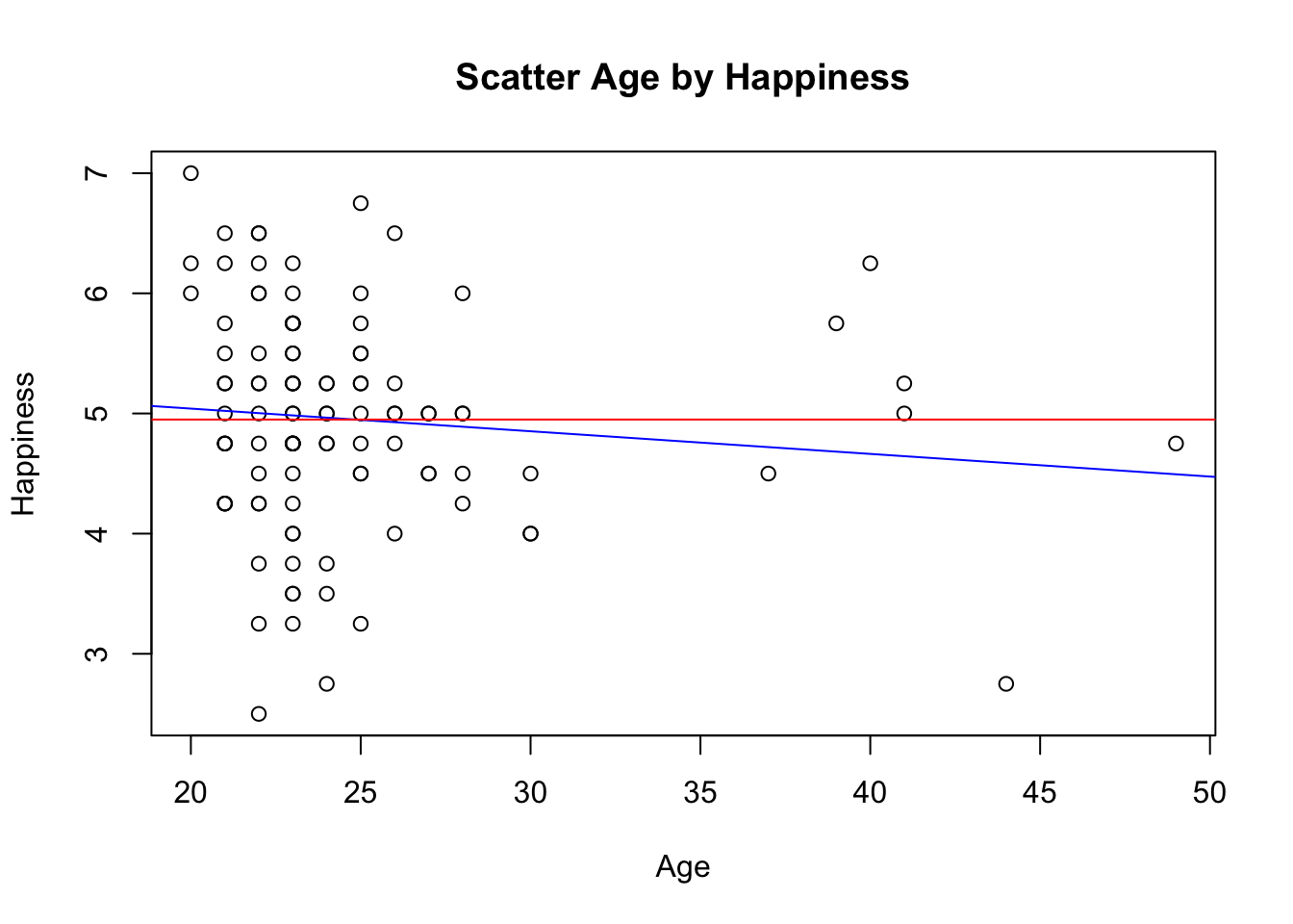

3.4 Statistical Inference

3.4.1 Basic Concepts

At this point we know that:

$b_1=-0.02$, meaning that for every year our sample gets older it gets less happier by $-0.02$;
$PRE=0.01$, meaning that the proposed model with age $\bar{Happiness}_i=b_0+b_1*Age_{i}$ is $1\%$ better than the null model $\bar{Happiness}_i = b_0$ in reducing the error (in other words we can say that the proposed model is better by $1\%$ than the null model in accounting for the variance of Happiness).

Statistical inference is method that allows to determine if the estimates produced for our sample (i.e., $b_1=-0.02$ and $PRE=0.01$) can be generalized to the the population where the data was collected. In other words, it is the method to test the likelihood of an estimate for our sample to happen by chance if the value is generalized to the population. In our case, this means:

How likely is the variation of $0.02$ across age in our sample to result form chance?
How likely is the difference in error of $1\%$ between the null and the proposed model in our sample to result from chance?

Here we will study one of the most popular method of statistical inference - the Hypotheses Testing.

3.4.1.1 Hypothesis Testing

The hypothesis testing compares two hypothesis: one hypothesis for a proposed effect, $H_1$, which states that the effect in our sample did not happen by chance, with a corresponding null hypothesis, $H_0$, which sates that the effect in our sample happened by chance. If a given effect is likely to have happened by chance, we don’t reject $H_0$. Alternatively, if a given effect is not likely to have happened by chance, we reject $H_0$. The hypothesis testing method relies on two important (and often misinterpreted) statistical concepts: the test statistic and the p-value.

3.4.1.2 Test Statistic

The test statistic corresponds to a transformed value of the effect we are testing from its original unit into t or F values.The transformation of an effect into t or F values is done through a simple ratio between the estimation of the effect and the error associated with that estimation of the effect. The general formula for transforming an effect into a test statistic looks like this:

\[Test\;Statistics=\frac{effect}{random\;error}\]

Test statistics for $PRE$ and $b_1$ correspond to F and t statistics, respectively and can be computed using the following formula:

\[F=\frac{SSE_{reduction}/(p_{proposed}-p_{null})}{SSE_{proposed}/(N-p_{null})}\]

$SSE_{reduction}$ is the reduction of the sum squared errors;
$SSE_{proposed}$ is the sum squared errors of the proposed model;
$SSE_{null}$ is the sum squared errors of the null model;
$p_{proposed}$ number of parameters to compute the full model
$p_{null}$ number of parameter to compute the null model.

\[t=\frac{b_1}{SE_{b_1}}\]
\[SE_{b_1}=\frac{s_e}{\sqrt{SSE_X}}\]

$SE_{b_1}$ is the standard error of $b_1$;
$s_e$ is the standard deviation for the full model;
$SSE_X$ is the sum of squared errors of the independent variable.

3.4.1.3 P-Value

Test statistic values are so important because they can be represented in the corresponding theoretical distribution and determined the likelihood of happening by chance. Theoretical distributions of test statistic values are continuous distributions of probability of chance:

The more extreme the test statistic value, the less likely this value is to happen by chance;
The less extreme the test statistic value, the less likely it is to happen by chance.

Here are two examples of these theoretical distributions with the corresponding frequency for the t and F values plotted in the $X$ axis is given in the $Y$ axis. Probabilities (i.e., likelihood) in density functions like these are given by areas (i.e., specific intervals of t and F values).

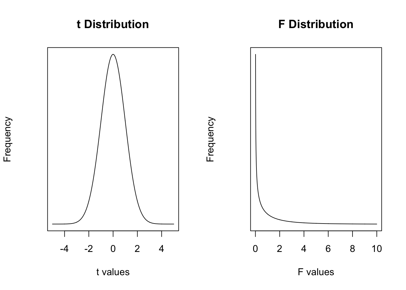
The p-value is nothing more than the probability of obtaining test statistic value equal or the most extreme to the one that is associated with the effect being tested for generalisability.

3.4.1.4 Significance Level

The significance level corresponds to chance probability that the researcher considers low enough so that we can say that a certain estimated effect did not happen by chance. There is a convention among scientists where only when the p-value is equal to or less than 0.05 it can be said that an effect did not occur by chance. In practice, applied to the hypothesis testing:

if the $p-value\leq0.05$, we reject the null hypothesis and consider that the effect is statistically significant;
if the $p-value>0.05$, we do not reject the null hypothesis and consider that the effect is not statistically significant.

3.4.2 In Practice

Here we will not compute test statistics values by hand nor using the F and t tables to match the test statistic with the corresponding p-value. Here we run the appropriate statistical test and look for the corresponding test statistics and p-value on the output. Run a simple linear regression using the summary() aov() and the anova() look at the test statistic of $PRE$ and $b_1$.

summary(Model.1) # estimates

## 
## Call:
## lm(formula = Happy$HappyScale ~ Happy$Age)
## 
## Residuals:
##      Min       1Q   Median       3Q      Max 
## -2.50321 -0.45605  0.04395  0.55338  1.95907 
## 
## Coefficients:
##             Estimate Std. Error t value            Pr(>|t|)    
## (Intercept)  5.41819    0.44337  12.220 <0.0000000000000002 ***
## Happy$Age   -0.01886    0.01748  -1.079               0.283    
## ---
## Signif. codes:  0 '***' 0.001 '**' 0.01 '*' 0.05 '.' 0.1 ' ' 1
## 
## Residual standard error: 0.9073 on 102 degrees of freedom
## Multiple R-squared:  0.01129,    Adjusted R-squared:  0.001592 
## F-statistic: 1.164 on 1 and 102 DF,  p-value: 0.2831

aov(Model.1) # SSE

## Call:
##    aov(formula = Model.1)
## 
## Terms:
##                 Happy$Age Residuals
## Sum of Squares    0.95838  83.96410
## Deg. of Freedom         1       102
## 
## Residual standard error: 0.9072913
## Estimated effects may be unbalanced

anova(Model.1) # detailed SSE

## Analysis of Variance Table
## 
## Response: Happy$HappyScale
##            Df Sum Sq Mean Sq F value Pr(>F)
## Happy$Age   1  0.958 0.95838  1.1642 0.2831
## Residuals 102 83.964 0.82318

3.4.2.1 Inference for $PRE$

The statistical inference for $PRE$ tests the likelihood of the reduction of the error of the proposed model relative to the the null model observed in the sample (the $R^2$ value) happening by chance if the value is generalized to the population. The statistical hypothesis for this inference is given by the following notation:

\[H_0:\eta^2=0\;vs\;H_1:\eta^2\neq0\]

$H_0$ corresponds to the null hypothesis and states that the the reduction of the error of the proposed model observed is the sample ($R^2$) is likely to have happened by chance if the value is generalized to the population ($\eta^2$).
$H_1$ corresponds to the alternative hypothesis and states that the the reduction of the error of the proposed model observed is the sample ($R^2$) is not likely to have happened by chance if the value is generalized to the population ($\eta^2$).

The value of the test statistic and the corresponding p-value for this inference is $F=1.16$ and $p-value=0.28$. Considering that $p-value>0.05$, the test statistics has a high likelihood of happening by chance. Consequently, the decision for this test is that we don’t reject $H_0$, meaning that the reduction of the error of the proposed model relative to the the null model observed in the sample is not statistically significant.

3.4.2.2 Inference for $b_1$

The statistical inference for $b_1$ tests the likelihood of the difference in happiness between man and woman observed in the sample (the effect of age represented by $b_1$) happening by chance if the value is generalized to the population. The statistical hypothesis for this inference is given by the following notation:

\[H_0:\beta_1=0\;vs\;H_1:\beta_1\neq0\]

$H_0$ corresponds to the null hypothesis and states that the effect of age ($b_1$) is likely to have happened by chance if the value is generalized to the population ($\beta_1$).
$H_1$ corresponds to the alternative hypothesis and states that the effect of age ($b_1$) is not likely to have happened by chance if the value is generalized to the population ($\beta_1$).

The value of the test statistic and the corresponding p-value for this inference is $t=-1.08$ and $p-value=0.28$. Considering that $p-value>0.05$, the test statistics has a high likelihood of happening by chance. Consequently, the decision for this test is that we don’t reject $H_0$, meaning that that the effect of age observed in the sample is not statistically significant.

3.5 Model Estimation and Statistical Inference Conclusion

Experienced Researchers report promptly the results of the model estimation, they don’t need to estimate in detail the null a proposed models nor the hypothesis testing process. These serve as a demonstration of the origin and meaning of the concepts of model, error, effect, test statistic and p-value in the context of the simplest type of proposed model. Here is an example of how to write down the results.

With our research question we what to determine whether age is a good predictor of happiness. To test this we ran a simple linear regression. The results indicate that the age variable reduces the error by $1\%$ but this effect is not statistically significant with $F=1.16$ and $p=0.28$. Additionally, the analysis of the estimated parameters indicates that for each year of age the level of happiness decreases by $0.02$ but, as already noted by the analysis of the model performance, this is effect is not statistically significant, $t=-1.08$, $p=0.28$.

3.6 Knowledge Assessment

Here is what you should know by now:

What is the proposed model;
What is proportion of the reduction of the error;
The relevant effects in model with one independent variable;
The hypothesis testing procedure;
What is a test statistics;
What is a p-value;
What means to say that an effect is statistically significant.
What are the appropriate statistical tests to model the effect of a quantitative independent variable on a quantitative dependent variable.

3.7 More About… interpreting effects in linear modeling

A proposed model like this $\bar{Happiness}_i = b_0+b_1age_{i}$ has two effects:

The overall effect of the model, given by the PRE;
The specific effect of age given by parameter b1.

3.7.1 What is the meaning of $b_0$?

Linear modeling can give bizarre results - in the case of our proposed model, $b_0=5.42$ corresponds to the estimated happiness level when age is 0 years! The idea of our research problem was not to estimate the happiness of children, but rather to estimate happiness in older age groups. Linear regressions will make this type of estimation, and it is the researcher that has to decide what is and what is not important. The parameter $b_0$ is not an important parameter to answer our research question. There are research questions in which the $b_0$ can be used but it is not common and it is not the case of the research problem that we are working here.

3.7.2 What is the diference between $PRE$ and $b_1$ in our model?

The overall effect of the model given by PRE and the effect of age given by b1, in the of Model I, redundant because any reduction in the error of the proposed model is due to the effect of age! A demonstration of this is that the statistical value of the PRE $F=1.16$ is equivalent to the square of the test statistic of b1 $t=-1.08$. This makes sense because PRE is measured in square happiness (the SSE) and b1 simply in happiness and the test statistics used account for that (the F distribution is a squared t). In this line, you can also see that the p-value of PRE and b1 are exactly the same $p-value=0.28$. Note that, a corollary form this rational is that if the overall effect of the model PRE is not statistically significant, none of the independent variables (in this case Age) will be statistically significant.

3.7.3 What is the meaning of the symbols used in the enumeration of the hypothesis?

The hypothesis $PRE$ are enumerated like $H_0:\eta^2=0\;vs\;H_1:\eta^2\neq0$ and for $b_1$ enumerated like $H_0:\beta_1=0\;vs\;H_1:\beta_1\neq0$.The usage of the Greek symbols to refer to the estimates is to state that we are testing the inference that the parameter estimate from our sample can be generalized to the population. The $\neq$ sign has two different interpretation. In the case of PRE, because it is a squared value, it can only take positive values, and so it is either $=0$ or $>0$. Still, notation wise, we used the the format about ($=$ versus $\neq$). In the case of parameter estimates, it is more complex because the values can take positive or negative values. In this case we refer to $H_1$ as differing from $0$ because we had no specific expectation about the direction of the effect. More specifically, we did not have a specific hypothesis about if age would increase or decrease happiness!

Step by Step I: Linear Models