Chapter 2 Supply
2.1 Learning outcomes
At the end of this chapter you should be able to
- Understand and use the WS-PS model
- Explain the properties of the Phillips curve and discuss why this relationship has become weaker in recent years
- Analyse the determinants of medium term unemployment
- Outline the economic consequence of divergence from medium-term equilibrium

Work
Supply is about firm decisions concerning the level of output, employment as well as wages and prices. The labour market does not appear to work like a traditional market that are determined by supply and demand. Unemployment is characteristic of a capitalist economy. Workers are willing to work at the prevailing wage rate but cannot find a job. Across the world this is happening but the supply-demand model suggests that the wage will fall to clear the market. Unemployment varies from country to country and across time, so it is clear that the business cycle and institutions can affect the number of people without a job. The unemployed are not happy to be without a job. (Clark and Oswald 1994) found that unemployed workers have twice the amount of mental distress as the employed. This is not volentary unemployment.
2.2 Why do labour markets not clear?
The New Keynesian model uses an efficiency wage model for the labour market (Carlin and Soskice 2015). This allows us to explain unemployment and the failure of wages to clear the labour market. The supply of labour is determined by the wage setting (WS) curve. The higher the wage, the more willing people are to work. The demand for labour is shown by the price setting (PS) curve. Firms offer wages based on the level of productivity, the level of competition, taxes and other factors. You can revisit the CORE textbook for more details on the labour market supply model.
Efficiency Wage model (Carlin and Soskice 2015)
The efficiency wage idea was first proposed by (Shapiro and Stiglitz 1984) in a paper called Equilbrium Unemployment as a Worker Discipline Device.
The model for the supply side of the economy is also based on monopolistic-competition where firms have market power to set prices. There can be changes in the level of competition based on the number of firms in an industry. The greater the market power, the more firms are able to increase their mark-up or profit margins. At the extremes, there are perfectly competitive and monopolistic markets.
It is assumed that wages and prices are not adjusting continuously but are changed infrequently. (Barattieri, Basu, and Gottschalk 2010) analysed wage setting in the US and found that wages were sticky. A simple model would suggest that wages are set once a year. This does not appear to vary much across different industries. (C. Campbell and Kamlani 1997) surveyed 184 firms and found that most firms were reluctant to cut wages in a recession. Firms felt that they would lose their best workers. Firms also thought that it would damage moral and reduce effort. (Bewley 2007) review literature on wage rigidity and fairness and found that wage cuts were only perceived as being fair if they saved a large number of jobs. This may explain why wages do not tend to fall to clear the market during a recession. However, rigidities in price setting varies by industry.
Nominal wages do not adjust immediately to fluctuations in aggregate demand. Economic agents set wages and prices with a target real value that requires some assumption about future inflation. The real wage (w) is the nominal wage (W) deflated by the price level (P).
\[w = \frac{W}{P}\]
For this New Keynesian model, wages are set once a year during the wage round and prices are adjusted after that. Therefore, wages and prices adjust to aggregate demand with a lag. In this case a positive demand shock will lead to higher employment, lower unemployment and an increase in wages (as a move up the WS curve). Firms respond with an increase in prices. We assume that the mark-up or profit-margin is unchanged. All firms in the industry increase wages.
2.3 Changes in equilibrium unemployment.
Equilibrium unemployment will rise if the WS curve shifts upwards or the PS curve moves downwards.
An increase in unemployment benefits would shift the WS curve upwards. There is a trade off between the effect that an increase in benefits has on reducing the cost of job losses and the need to shift to a lower point on that wage setting curve to ensure productive output. This is achieved with a higher level of unemployment.
Higher mark-ups as a result of lower competition. The PS curve is reduced and a higher share goes to profits. There is less employment and lower real wages. This may be something to consider with recent examples. With the higher cost of job loss the real wage is lower.
Policies that shift the WS or PS curves will affect the level of equilibrium unemployment and the growth rate of the economy. These are supply side policies that we will focus on in Chapter .
2.3.1 Labour-supply
Analysis of the supply-side of the economy is broken down into two parts: supply-side effects on unemployment; nominal rigidities.
\[w = Pe B(N, z)\]
Where the wage \((W)\) is determined by the expected price level, the level of employment \((N)\) and a set of wage-push variables \((Z).\) This will include changes in benefits and the presence of unions.
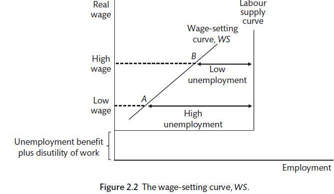
Though nominal wages are set or negotiated, works are interested in the real wage. The wage-setting (WS) real-wage equation is
\[w(WS) = W/Pe = B(N, Z)\]
The opportunity cost of taking a job is dependent on two factors: benefits and the disutility of working. The wage is above the opportunity cost of working and increases as the unemployment rate falls. As unemployment falls firms have to pay more to get people to work hard as there are lots of job opportunities. There are a number of enhancements that can be applied, including adding monopoly unions. As such, changes in institutions can affect the WS curve and the equilibrium level of unemployment.
2.3.2 Labour-demand
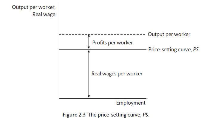
In a competitive market the firm sets prices and the quantity of labour required with reference to the marginal product of labour. In this case \(P = MC and W/P = MPL\). However, once there is market power, as is the case with our assumption of monopolistic competition, firms facing a downward-sloping demand curve will produce to maximise profits. The mark-up on marginal cost will be depend on the elasticity of demand, which will be influenced in a positive direction by the level of competition. As elasticity rises the mark-up will fall. A horizontal PS curve is usually employed, if firms set prices according to a mark-up over costs. Now the fixed output per worker is split between profit per worker and the real wage per worker. The real wage is the marking-up of unit labour costs by a fixed percentage \((\mu)\).
Therefore,
\[P = (1 + \mu)(W/\lambda)\]
Where \(\lambda\) is output per worker \((y/N)\).
Output per worker is divided into real wages per worker and real profits per worker.
Productivity, prices and wages
There is a divergence between the real consumption wage (based on post-tax income and excise duties prices) and the real product wage that is paid by the employers - including income tax and other taxes relative to the price that is received for product after indirect taxes are paid. The difference is the tax wedge. The tax wedge is one of the price-push factors that may affect the PS wage.
\[W^PS = \lambda F (mu, z)\]
Changes in productivity, competitive conditions and taxation can change the price-setting wage. Other price-push factors are business regulations and employment relations, Some health and safety regulations may impose costs but provide an offsetting increase in productivity.
Labour market equilibrium is at the intersection of the upward sloping WS curve and a flat or downward sloping PS curve.
\[W^ws = W^ps\]
\[B(N, z_w) = \lambda F (\mu, z_p)\]
2.4 Exercise
Please go to the labour market app and make the following adjustments:
An increase in productivity
A reduction in benefits
An increase in competition
Make sure that you are happy with the model and the adjustments to real wages, employment and unemployment that each of these changes would suggest. In what ways is the model unrealistic? How can we account for that? How would those changes affect the model?
2.5 The labour market and the business cycle
Nominal rigidities describes the way that wages and prices fail to constantly change and clear the market. A model where workers demand wage changes based upon the level of unemployment and firms accept these wage changes and then adjust prices so that the mark-up over costs is maintained is supported by empirical evidence (Alvarez et al. 2006). As a result, employment will change with the business cycle - rising when the economy is strong and falling when it is weak. Firms often set prices strategically in relation to the behaviour of other firms in the industry.
Okun's Law studies the empirical relationship between unemployment and output. The relationship may be affected by labour hoarding and by movement into and out of the labour force. A 1% change in output above or below its long run trend has an effect of 0.5 percentage points on the unemployment rate. This is different for different countries. A formalisation of the link between unemployment and inflation is the behavioural model called the Phillips curve. This can be written as
\[W^ws(y) = (W/P)^ws = B + \alpha (y_t - y_e) + z_W\]
Where B is a constant that reflects unemployment and the disutility of work while Z_W is a set of cost-push factors, \(y_t\) is the level of output or GDP and \(y_e\) is the equilibrium output associated with the natural or long-run level of unemployment.
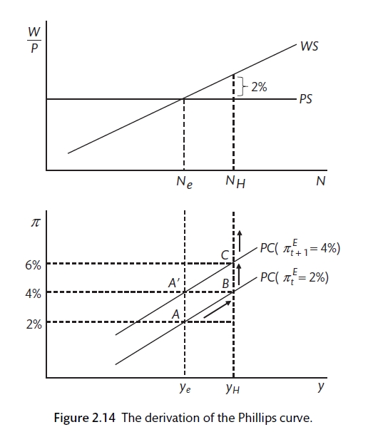
2.6 The Phillips curve
You can revisit the CORE discussion of the Phillips curve. In the New Keynesian model, the Phillips curve is pinned down by lagged inflation because lagged inflation is a key component of the wage inflation mechanism. This is because we assume that inflation expectations are based primarily on the past performance of inflation. We will use adaptive wage expectations. When determining the wage that they will accept, workers look at past inflation as their guide to the future. We can adjust this assumption if necessary.
This is the adaptive expectations Phillips curve.
\[\pi_t = \pi_t^E + \alpha (y_t - y_e)\]
The Phillips curve (Carlin and Soskice 2015)
2.7 Demand and supply shocks
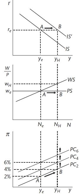
We can use the components that we have of the New Keynesian model to discuss the effect of demand and supply shocks. The demand shock could be the fall in spending that has been caused by the Covid-19 lockdown or by an increase in household spending due to increased confidence about the future. The IS curve shifts, the increased demand and output causes a disequilibrium in the labour market and inflationary or deflationary pressure. There is nothing to stop inflation rising or falling in without intervention from the central bank.
A demand shock (Carlin and Soskice 2015)
There are a number of factors that could produce a supply shock: technology or productivity shock \((\lambda)\), a shift in worker bargaining power (WS) or a change in level of competition amongst firms(PS). UK labour market reforms of the 1980s included reducing trade union power, making it more difficult to apply for unemployment benefit and reducing the level of benefit. These have the effect of shifting the WS curve to the right and reducing the equilibrium level of unemployment.
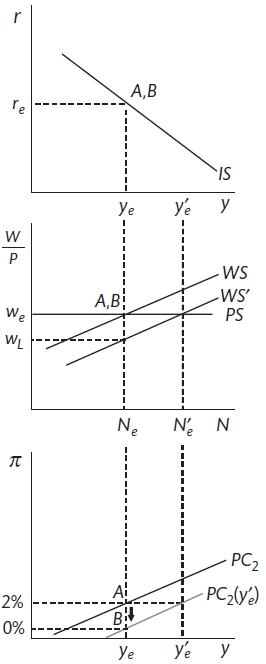
A supply shock (Carlin and Soskice 2015)
A shift in the WS curve means that employment at \(N_e\) is below the new equilibrium of \(N_e^1\). This will cause workers to accept lower wage increases and for inflation to fall as these cost changes feed through into prices. The process will unless demand and output can increase employment to the new equilibrium.
References
Alvarez, L.J., E. Dhyne, M. Hoeberichts, C. Kwapil, C. Le Bihan, P. Lnnemann, F. Martins, et al. 2006. “Sticky Prices in the Euro Area: A Summary of New Micro-Evidence.” The Journal of Economic Perspectives 4 (2/3): 575–84.
Barattieri, A., S. Basu, and P. Gottschalk. 2010. “Some Evidence on the Importance of Sticky Wages.” NBER Working Paper, no. 16130.
Bewley, T. 2007. “Wages Don’t Fall During a Recession.” In Behavioural Economics and Its Applications, edited by Peter Diamond and Hannu Vartiainen, 157–88. Princeton, NJ: Princeton University Press.
Campbell, C.M., and K.S. Kamlani. 1997. “The Reasons for Wage Rigidity: Evidence from a Survey of Firms.” The Quarterly Journal of Economics 112 (3): 759–89.
Carlin, W., and D. Soskice. 2015. Macroeconomics: Institutioins, Instability, and the Financial System. 1st ed. OUP.
Clark, A.E., and A.J. Oswald. 1994. “Unhappiness and Unemployment.” The Economic Journal 104 (424): 648–59.
Shapiro, C., and J.E. Stiglitz. 1984. “Equilibrium Unemployment and a Worker Discipline Device.” The American Economic Review 74 (3): 433–44.