Chapter 11 Extending the open economy model
By the end of this chapter you should understand the following:
The role of policy is oil and other supply shocks
The intertemporal balance of payments model
The source of sustained financial imbalances
There are two major issues to be explored with the Medium Run model: changes in import prices; international imbalances.
11.1 Supply shocks
A supply shock is defined as a terms of trade shock that changes the relative price of manufacturing goods and raw materials. This shock will tend to affect the AD curve, the ERU curve and the BT curve, shifting them to the left. For example, a rise in the price of oil means that the relative price of oil to manufacturing goods become more expensive.
\[\tau = \frac{P^*_{rm}}{P^*_{mf}}\]
The price setting curve is defined for a given real exchange rate and \(P^*_{rm}\) is defined as the overseas price of raw materials and \(P^*_{mf}\) is defined as the overseas price of manufactured goods.
\[Q = \frac{p^*_{mf}e}{P_{mf}}\]
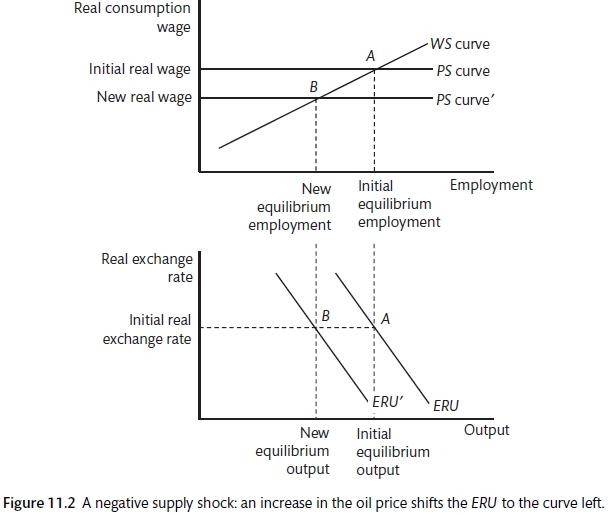
If the price of oil rises relative to manufactured goods (\(\tau \uparrow\)), this will be passed on as higher consumer prices and a lower real wage for consumers as firms protect their profit margins. The price setting curve shifts downwards and the ERU curve shifts to the left. A simple way to model this is to assume that all imports are oil and the consumer price index is the price index of home value added (i.e. the mark-up over unit labour costs and the cost of imported oil).
\[P_t = P_{mf} + v \tau P_{mf}^* e\]
where
\[P_{mf} = \frac{W}{(1 - \mu)\lambda}\]
And v is the unit material requirement. Therefore,
\[W^{PS} = \frac{(1 - \mu)\lambda}{1 + v\tau Q}\]
Where \(\mu\) is the price mark-up over unit labour costs, \(\lambda\) is productivity and \(v\) is the share of raw materials in production. So any rise in \(\tau\) reduces the real wage (though this could be offset by a fall in v).
Given this framework, a rise in oil has three effects: that on AD, that on the trade balance and that on supply (ERU).
Aggregate demand and trade are affected in the same way: the rise in the price of imports reduces the income left for other goods. This shifts the AD curve and the BT curve leftwards. We can assess the trade balance from Chapter 10 with the terms of trade \((\tau)\) added.
Since the import price of manufactured goods is
\[P_M = P^*_{mf}e\]
and is
\[P_M = \frac{P^*_{rm}P^*_{mf}e}{P^*_{mf}}\]
when imports are raw materials, imports in real terms (M) are
\[M = \left ( \frac{P^*_{rm}P^*_{mf}e}{P^*_{mf}P_M} \right ) M(Q, y) = \tau QM(\tau Q, y)\]
Everything else equal, a rise in \(\tau\) increases the import bill, depressing net exports,
\[X - M = X(Q, ^*) - M(\tau Q, y)\]
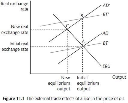
Oil is an important part of the household consumption bundle and a key input into the production process. A rise in oil prices will result in a shock for an oil consuming nation: prices are higher so the cost of imports rises. This will shift the AD curve to the left and will shift the BT line to the left. The initial shock leads to a depreciation of the real exchange rate that compensates for the price rise, the new AD and new BT curves intersect at the same level of output. However, there is also a supply shock as the consumer price index rises, this is represented in a lagged move to the left in the ERU curve. As consumer prices rise, the PS curve shifts downwards.
labour market and import prices (Carlin and Soskice 2015)
11.2 Oil shocks and policy responses
In the 1970s, the policy response to the oil shock was to focus on the demand shock and ignore the supply shock. As a result there was upward pressure on inflation and rising unemployment. There is a gap between the WS and PS curves, inflation is rising. Policy-makers attempt to offset the demand shock by using policy to push the AD curve back to the original position. If the economy gets back to a position of stable inflation, this is at the cost of higher unemployment and a significant deterioration in the trade position. The government's fiscal position will also have been damaged in order to boost AD. Using monetary policy or exchange rate depreciation has the same effect of attempting to hold the economy above the equilibrium at which inflation will remain constant.
A better response to this type of shock would be a supply side measures, such as a wage accord. This could shift the WS curve downwards and provide a partial offset to the movement of the PS curve. If the wage accord is complete, the ERU curve will not shift. However, this policy is difficult to achieve as the combination of wage restraint and rising oil prices means that there is a fall in living standards. It might be presented as an exchange of employment for wage restraint. This sort of tripartite agreement between government, unions and employers is more likely in the German or Scandinavian labour model.
The third oil shock in the 2000 to 2005 period when oil price gains did not lead to stagflation? Policy-makers were more away of supply=shocks than they were in 1973. Labour markets appear to have changed and workers were unable to seek compensation for the increase in oil pries. Confrontational unions had become less important. Real wages tended to fall. Banks were much more willing to lend to compensate for any decline in real wages as a result of the oil price rise. As we know, people in countries like the UK, the US and Spain were able to borrow against the value of their houses to maintain consumption in the face of falling real wages. This meant that the ERU and AD curves moved a lot less in this period.
Supply shock and the medium-run model (Carlin and Soskice 2015)
11.3 Current account imbalances
It is possible to look at current account and global balances in the same way that we discussed household balances. Just as households can borrow against future income to improve welfare, it is also possible that a country with a resource find could borrow against this before the proceeds are received by running a current account deficit. However, it is also possible that a country with consumer boom may run up a current account deficit. In this case the increased borrowing from abroad is not being offset by expected increase in future income. The run up to the 2008 financial crisis was accompanied by an increase in global imbalances: while UK, Spain, US and Ireland saw current account deficits rise, China and Germany experienced increased surplus. The Japanese surplus remained large. The two-block model will allow an analysis of these issues.
The fall in \(X - M\) pushes the BT and AD curves to the left. There is an immediate depreciation with no change in output. However, with the shift in AD, this is an inflationary state and there is a gradual adjustment back to the point where the lower level of output is consistent with the stable inflation, trade balance and exchange rate stability.
The current account can be treated like an inter-temporal issue.
\[X - M = y - C - I - G\]
\[CA = X - M + INT\]
where INT equals net interest (income) from abroad
\[CA = y + INT - C - I - G = \tilde{y} - C\]
where \(\tilde{y}\) is aggregate household disposable income (savings plus taxes).
The inter-temporal current account (ICA) is a forward-looking version. The cumulative outcome of past current accounts will be the net foreign assets (NFA). The model is based on two assumptions: perfect capital mobility and substitutability; forward-looking, rational, consumption-smoothing households, with infinite horizons. Using the notation of the household
\[CA = \sum_{t=1}^{\infty} \frac{1}{1 + r} \gamma \Delta \tilde{y}_{t+i}\]
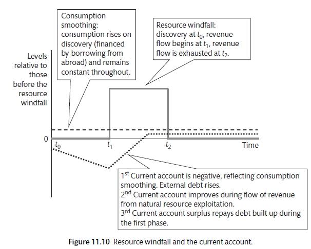
Current account positions lead to fluctuations in NFA. This is the equivalent of households becoming more indebted in the standard model. Countries smooth consumption due to fluctuations in expected future income. For example, a country that finds a new natural resource should experience an increase in current consumption and investment, a current account deficit and an appreciation of the real exchange rate. Consumption is smoothed, there is borrowing from abroad (current account deficit) and the exchange rate rises to the rate that will balance the current account in the long run. A current account deficit may also be caused by countries finding that there are better investment opportunities abroad. High savings countries in Asia may be examples of this.
Balance of Payments and Consumption Smoothing (Carlin and Soskice 2015)
11.4 Sectoral Financial Balances
One way to look at the current account is as a component of overall sectoral financial balances. This can be used to discuss national or global imbalances. It is possible to consider what would have to change in order for the surplus or deficit to be eliminated. The private sector balance and the public sector balance must be equal to the trade position (assuming away net earnings from abroad for now).
\[(S - I(r^*)) + (T - G) = X - M\]
Or
\[(s_1y^{dis} - c_0 - I(r^*) + (ty - G) = X(Q, y^*) - QM(Q, y)\]
11.5 Global imbalances and the GFC
The build up to the GFC was characterised by large scale global imbalances. (Caballero, Farhi, and Gourinchas 2008) modelled a world of three groups: the first is fast growing with well developed financial systems; the second is slower-growing and less developed financial systems; finally, fast growing a undeveloped. The group of emerging economies could not find sufficient domestic assets to satisfy their savings needs, these are supplies by the first group. The first group is the US (with the UK and Australia), the second is Germany and Japan and Korea, the final group is China and other developing countries, including at times the major oil exporters.
Two Country Model (Carlin and Soskice 2015)
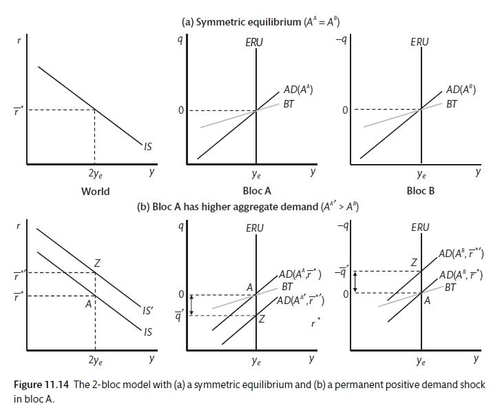
A two block model seeks to explain how persistent imbalances can exist in the medium term. To focus on the interaction of the two blocks, there is an abstraction away from the downward sloping ERU curve. It is assumed that there are two blocks: A represents the current account deficit countries and B are the current account surplus countries. They have inflation-targeting central banks and there is a set interest rate \((r = r^*)\) and real exchange rate \((q = \bar{q})\). Assume that the IS coefficients on real interest rates and the real exchange rate are the same for A and B and equal to one.
\[y_A = A^A + r^* + \bar{q}\]
\[y_B = A^B + r^* + \bar{q}\]
\[q = log \left ( \frac{P^*e}{P} \right )\]
\[e = \frac{\$_A}{\$_B}\]
If we assume that \(A^A > A^B\) due to the higher growth of the surplus countries,
\[A^A - i^* + \bar{q} = A^B - \bar{q}\]
\[2\bar{q} = A^A - A^B\]
\[\bar{q} = \frac{A^B - A^A}{2} < 0 \]
Block A's real exchange rate is appreciated and there is a trade deficit that is equal to the trade surplus of B,.
\[BT^A = y_e - (A^A - i^*) = \bar{q} < 0 \]
\[BR^B = y_e - A^B - i^*) = \bar{q} > 0\]
The real exchange rate ensures that demand on aggregate between the two blocks is appropriate. Note that the real interest rate \((i^*)\) adjusts to ensure that demand is consistent with output. If demand is block a is \(y^{da}\)
\[y^{da} + y^{db} = 2y_e\]
Hence from the IS
\[A^A - i^* + \bar{q} + A^B - i^* - \bar{q} = 2y_e\]
or
\[i^* = \frac{A^A + A^B}{2} - y_e\]
The world interest rate maintains balance because central banks in the two regions set interest rates to maintain inflation balance in their respective countries.
References
Caballero, R., E. Farhi, and P.O. Gourinchas. 2008. “An Equilibrium Model of Imbalances and Low Interest Rates.” The Amercial Economic Review 98 (1): 358–93.
Carlin, W., and D. Soskice. 2015. Macroeconomics: Institutioins, Instability, and the Financial System. 1st ed. OUP.