Chapter 13 Monetary policy

By the end of this chapter you should understand:

• The evolution from monetary to inflation targeting

• The modern monetary framework and some alternatives

• The use of alternative monetary measures as a consequence of the zero bound

The classical dichotomy is the contrast between the real and nominal economy. In a perfectly competitive economy wages and price adjust immediately to maintain equilibrium; preferences and technology determine household and firm behaviour; money determines the price level. The Quantity Theory of Money encapsulate the classical dichotomy. This is essentially the Real Business Model. This is the main alternative to the New Keynesian model.

\[Py = Mv\]

Where P is the price level, y is output, M is the quantity of money and v is the velocity of circulation.

\[\frac{\Delta{P}}{P} + \frac{\Delta{y}}{y} = \frac{\Delta{M}}{M} + \frac{\Delta{v}}{v}\]

Assuming that there is no growth and velocity is zero.

\[\frac{\Delta{P}}{P} = \pi = \frac{\Delta{M}}{M}\]

As prices adjust the economy is always at equilibrium \((y = y_e)\) and therefore the policy maker should just determine the price level by fixing the growth rate of money.

Germany and Switzerland made good use of monetary targets after the breakdown of Bretton Woods.

\[\pi_t = \left [ \chi \pi^T + (1 - \chi)\pi_{t-1} \right ] + \alpha (y_t - y_s)\]

Remember that \(\chi\) represents the degree of central bank credibility. It will range from zero to one, with one being complete credibility. The Bundesbank, the German central bank, was able to get a near unity value for the \(\chi\) parameter. Credibility allows the central bank to deal with shocks more swiftly and with less economic pain.

For monetary targetting to work the central bank must be able to control the money supply and there must be a clear link between money and nominal GDP. While this was the case with Germany, it was not the case with the US, UK and Canada. The UK provides a nice case study: the BoE could not control money supply (only base money) and the relationship between money and nominal GDP broke down. This provides a constraint on the value of \(\chi\) that is less than unity. Goodhart's law says that as soon as a monetary aggregate is targeted it is no longer any use as economic agents' knowledge of the target changes their behaviour.

These failures with money targets outside of Germany and Switzerland led towards the adoption of inflation targets. This is a more direct approach. Recall that the central bank minimises its loss function (inflation and output gap) relative to the Phillips curve.

Loss function \[L = (y_t - y_s)^2 + \beta(\pi_t - \pi^T)^w\]

Phillips curve \[\pi_t = \pi_0 + \alpha(y_t - y_s)\]

Monetary Policy Rule \[(y_1 - y_s) = \alpha \beta (\pi_1 - \pi^T)\]

The MR equation reveals an interest rate or Taylor rule (J.B.Taylor 1993). The Taylor Rule article is here

\[r_0 - r_s = 0.5(\pi_t - \pi^T) + 0.5(y_o - y_e)\]

Where \(r_s\) is the stabilisation rate and \(y_0 - y_e\) is the percentage gap. It is possible to create a best response rule for the central bank. The original Taylor rule was an empirical model. Using the three equations (with the deviation from IS).

\[\pi_1 = \pi_0 + \alpha(y_1 - y_e)\]

\[y_1 - y_e = -\alpha(r_0 - r_s)\]

\[(y_1 - y_e) = -\alpha\beta(\pi_1 - \pi^T)\]

\[\pi_0 - \pi^T = - \left (\alpha + \frac{1}{\alpha \beta} \right ) (y_1 - y_e)\]

Substitute \((y_1 - y_s)\) using the IS to get the interest rate rule

\[r_0 -r_s = \left ( \frac{1}{\alpha + \frac{1}{\alpha \beta}} \right ) (\pi_0 - \pi^T)\]

So

\[r_0 - r+s = 0.5(\pi+_0 - pi^T) \]

\[if \alpha = \alpha = \beta = 1\]

From this, the higher \(\beta,\) the more the central bank's loss function hates inflation and the more the central bank should respond to inflation being above target; the higher \(\alpha\) the steeper the Phillips curve and the flatter the MR curve so output responds more and the central bank reaction will be less; as \(\alpha\) increases the IS curve gets flatter and AD is more responsive to interest rates and therefore the central bank needs less of a reaction to an inflation increase.

13.1 The monetary transmission mechanism

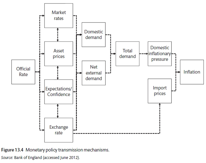
Bank of England chart (Carlin and Soskice 2015)

There are four main channels through which monetary policy affects the real economy: market rates; asset prices; expectations or confidence; the exchange rate. The BoE estimates that the effects of an interest rate change can take up to 1 year to affect output and that the rates can take up to 2 years to affect inflation. Though the central bank may have an inflation target or a duel-mandate, the focus on unemployment does not mean that they think that they can influence the equilibrium employment rate but rather there will be some trade off and a this may influence the choice of gradualist or shock-treatment policy. How are these differences reflected in actual behaviour?

13.2 Monetary response to bubbles

There is a question about how far the central bank should react to bubbles. Bubbles are painful because they cause price distortion and therefore a misallocation. They are also painful because the aftermath is usually lower output and employment. The Tech bubble of 2000 and the mortgage bubble of 2004-06 was not actioned by central banks. The policy was to deal with the aftermath. This is the so-called Greenspan Doctrine, named after the former head of the US central bank Alan Greenspan. He believed that it was difficult to identify bubbles and that it was easy to support the economy with monetary policy after a bubble burst. The period 2005-2008 showed that the last of these was not correct.

13.3 The zero bound

Using the Taylor Rule to assess monetary policy shows the importance of the lower bound as in most cases, it appears that negative interest rates should have been put in place. The Taylor Rule is assessed

\[i_t = \bar{i} + \gamma_1(\pi_t - \pi^T) + \gamma_2(y_t - y_e)\]

The following assumptions are made: \(\bar{i}\) is the average interest rate from 1999 to 2011; \(\pi_t\) is the core inflation rate (excluding food and energy) for the same period; \(\pi^T\) is the inflation target for the central bank; \(y_t - y_s\) is the output gap measured in percentage of potential GDP; \(\gamma_1\) is equal to 1.5; /gamma_2 is equal to either 1 or 1.5 so that different levels of unemployment aversion can be tested. Figure 13.5 shows the results for 1999 to 2011. The analysis shows that the US, Japan and the Eurozone all experienced the zero bound constraint. Japan has been constrained for 20 years. The UK experienced some inflation but this was due to the VAT increase and the fall in the value of the pound, the central banks took the view that this was a one-off change and did not react. The picture shows that conventional monetary policy may not work in these circumstances.

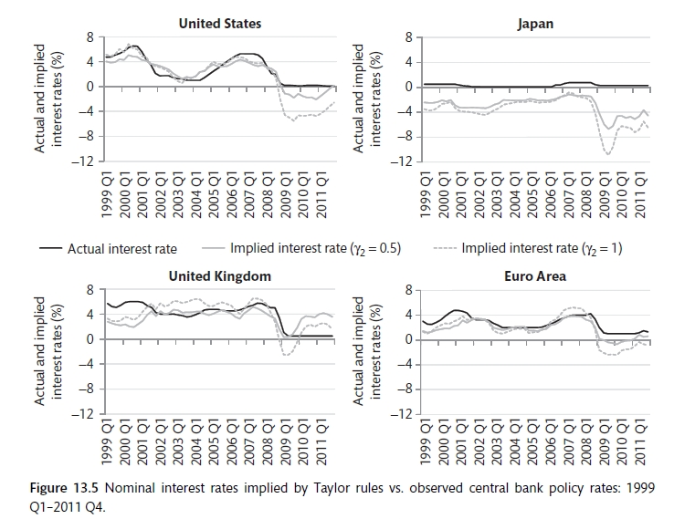
The Taylor Rule and the Zero bound (Carlin and Soskice 2015)

13.4 Alternative monetary policy

To combat the zero bound, the main policy used was quantitative easing. This involves using high powered money to purchase financial assets. In the UK the BoE bought government bonds from non-financial organisations, in the US it was mortgage-backed bonds bought from financial institutions. The transmission mechanism of monetary policy is more complex than that of the conventional policy. It could affect in a number of ways. The Bank of England believe that the transmission of unconventional monetary policy will come from the effect of an increase in asset pricing on borrowing costs and confidence. The aim is to reduce the wedge between the policy rate and the rate that households and incitations borrow at. QE also has a signalling effect. It shows that the central bank is serious about the inflation target. It is one way to fight against falling into the inflation trap. QE can encourage portfolio rebalancing. Sellers of bonds to the central bank will rebalance their portfolio, purchasing other risky assets and reducing their return as a result. QE can provide liquidity and reduce the liquidity premium. The policy will increase the amount of money in the economy.

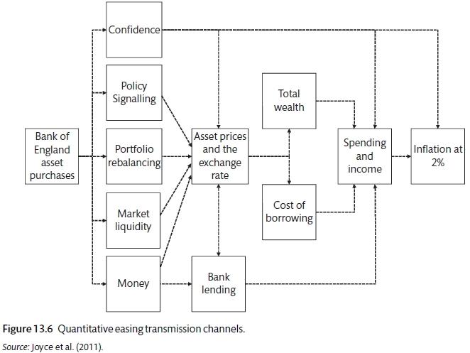
Alternative monetary transmission mechanism (Carlin and Soskice 2015)

The aftermath of the GFC has called into question the monetary policy framework that had gone before. There is increased focus on the limitation of the inflation-target approach and a desire to ensure that central banks take some action when borrowing and risk-taking is above the level that is seen to be socially optimal. As a result most central banks have started a more formal assessment of financial conditions.

There is also an awareness of the limitations of monetary policy under the zero-bound and of the way that government financial may swiftly deteriorate if they have been flattered by excessive taxation that is drawn from the financial industry during the financial acceleration phase. If this has been the case, government finances will swiftly deteriorate as the profitability of the financial sector is affected by the crisis.

References

Carlin, W., and D. Soskice. 2015. Macroeconomics: Institutioins, Instability, and the Financial System. 1st ed. OUP.

J.B.Taylor. 1993. “Discretion Vs Policy Rules in Practice.” Carnegie-Rochester Conference Series on Public Policy, no. 39. North-Holland: 195–214.