Chapter 2 Geographic data in R

Prerequisites

Note: this is the first edition of Geocomputation with R, first published in 2019 and with minor updates since then until summer 2021. For the Second Edition of Geocomputation with R, due for publication in 2022, see geocompr.robinlovelace.net.

This is the first practical chapter of the book, and therefore it comes with some software requirements. We assume that you have an up-to-date version of R installed and that you are comfortable using software with a command-line interface such as the integrated development environment (IDE) RStudio.

If you are new to R, we recommend reading Chapter 2 of the online book Efficient R Programming by Gillespie and Lovelace (2016) and learning the basics of the language with reference to resources such as Grolemund and Wickham (2016). Organize your work (e.g., with RStudio projects) and give scripts sensible names such as chapter-02.R to document the code you write as you learn.

The packages used in this chapter can be installed with the following commands:⁵

install.packages("sf")
install.packages("raster")
install.packages("spData")
remotes::install_github("Nowosad/spDataLarge")

If you’re running Mac or Linux, the previous command to install sf may not work first time. These operating systems (OSs) have ‘systems requirements’ that are described in the package’s README. Various OS-specific instructions can be found online, such as the article Installation of R 3.5 on Ubuntu 18.04 on the blog rtask.thinkr.fr.

All the packages needed to reproduce the contents of the book can be installed with the following command: remotes::install_github("geocompr/geocompkg"). The necessary packages can be ‘loaded’ (technically they are attached) with the library() function as follows:

library(sf)          # classes and functions for vector data
#> Linking to GEOS 3.9.0, GDAL 3.2.1, PROJ 7.2.1

library(raster)      # classes and functions for raster data

The output from library(sf) reports which versions of key geographic libraries such as GEOS the package is using, as outlined in Section 2.2.1. The other packages that were installed contain data that will be used in the book:

library(spData)        # load geographic data
library(spDataLarge)   # load larger geographic data

2.1 Introduction

This chapter will provide brief explanations of the fundamental geographic data models: vector and raster. We will introduce the theory behind each data model and the disciplines in which they predominate, before demonstrating their implementation in R.

The vector data model represents the world using points, lines and polygons. These have discrete, well-defined borders, meaning that vector datasets usually have a high level of precision (but not necessarily accuracy as we will see in Section 2.5). The raster data model divides the surface up into cells of constant size. Raster datasets are the basis of background images used in web-mapping and have been a vital source of geographic data since the origins of aerial photography and satellite-based remote sensing devices. Rasters aggregate spatially specific features to a given resolution, meaning that they are consistent over space and scalable (many worldwide raster datasets are available).

Which to use? The answer likely depends on your domain of application:

• Vector data tends to dominate the social sciences because human settlements tend to have discrete borders
• Raster dominates many environmental sciences because of the reliance on remote sensing data

There is much overlap in some fields and raster and vector datasets can be used together: ecologists and demographers, for example, commonly use both vector and raster data. Furthermore, it is possible to convert between the two forms (see Section 5.4). Whether your work involves more use of vector or raster datasets, it is worth understanding the underlying data model before using them, as discussed in subsequent chapters. This book uses sf and raster packages to work with vector data and raster datasets, respectively.

2.2 Vector data

Take care when using the word ‘vector’ as it can have two meanings in this book: geographic vector data and the vector class (note the monospace font) in R. The former is a data model, the latter is an R class just like data.frame and matrix. Still, there is a link between the two: the spatial coordinates which are at the heart of the geographic vector data model can be represented in R using vector objects.

The geographic vector data model is based on points located within a coordinate reference system (CRS). Points can represent self-standing features (e.g., the location of a bus stop) or they can be linked together to form more complex geometries such as lines and polygons. Most point geometries contain only two dimensions (3-dimensional CRSs contain an additional \(z\) value, typically representing height above sea level).

In this system London, for example, can be represented by the coordinates c(-0.1, 51.5). This means that its location is -0.1 degrees east and 51.5 degrees north of the origin. The origin in this case is at 0 degrees longitude (the Prime Meridian) and 0 degree latitude (the Equator) in a geographic (‘lon/lat’) CRS (Figure 2.1, left panel). The same point could also be approximated in a projected CRS with ‘Easting/Northing’ values of c(530000, 180000) in the British National Grid, meaning that London is located 530 km East and 180 km North of the \(origin\) of the CRS. This can be verified visually: slightly more than 5 ‘boxes’ — square areas bounded by the gray grid lines 100 km in width — separate the point representing London from the origin (Figure 2.1, right panel).

The location of National Grid’s origin, in the sea beyond South West Peninsular, ensures that most locations in the UK have positive Easting and Northing values.⁶ There is more to CRSs, as described in Sections 2.4 and 6 but, for the purposes of this section, it is sufficient to know that coordinates consist of two numbers representing distance from an origin, usually in \(x\) then \(y\) dimensions.

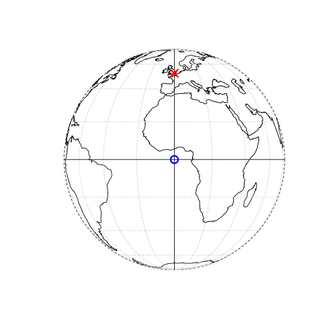
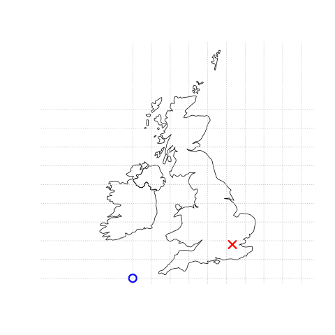
FIGURE 2.1: Illustration of vector (point) data in which location of London (the red X) is represented with reference to an origin (the blue circle). The left plot represents a geographic CRS with an origin at 0° longitude and latitude. The right plot represents a projected CRS with an origin located in the sea west of the South West Peninsula.

sf is a package providing a class system for geographic vector data. Not only does sf supersede sp, it also provides a consistent command-line interface to GEOS and GDAL, superseding rgeos and rgdal (described in Section 1.5). This section introduces sf classes in preparation for subsequent chapters (Chapters 5 and 7 cover the GEOS and GDAL interface, respectively).

2.2.1 An introduction to simple features

Simple features is an open standard developed and endorsed by the Open Geospatial Consortium (OGC), a not-for-profit organization whose activities we will revisit in a later chapter (in Section 7.5). Simple Features is a hierarchical data model that represents a wide range of geometry types. Of 17 geometry types supported by the specification, only 7 are used in the vast majority of geographic research (see Figure 2.2); these core geometry types are fully supported by the R package sf (E. Pebesma 2018).⁷

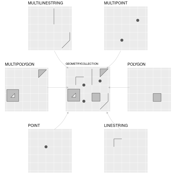
FIGURE 2.2: Simple feature types fully supported by sf.

sf can represent all common vector geometry types (raster data classes are not supported by sf): points, lines, polygons and their respective ‘multi’ versions (which group together features of the same type into a single feature). sf also supports geometry collections, which can contain multiple geometry types in a single object. sf provides the same functionality (and more) previously provided in three packages — sp for data classes (E. Pebesma and Bivand 2018), rgdal for data read/write via an interface to GDAL and PROJ (R. Bivand, Keitt, and Rowlingson 2018) and rgeos for spatial operations via an interface to GEOS (R. Bivand and Rundel 2018). To re-iterate the message from Chapter 1, geographic R packages have a long history of interfacing with lower level libraries, and sf continues this tradition with a unified interface to recent versions of the GEOS library for geometry operations, the GDAL library for reading and writing geographic data files, and the PROJ library for representing and transforming projected coordinate reference systems. This is a notable achievement that reduces the headspace needed for ‘context switching between’ different packages and enables access to high-performance geographic libraries. Documenation on sf can be found on its website and in 6 vignettes, which can be loaded as follows:

vignette(package = "sf") # see which vignettes are available
vignette("sf1")          # an introduction to the package

As the first vignette explains, simple feature objects in R are stored in a data frame, with geographic data occupying a special column, usually named ‘geom’ or ‘geometry.’ We will use the world dataset provided by the spData, loaded at the beginning of this chapter (see nowosad.github.io/spData for a list of datasets loaded by the package). world is a spatial object containing spatial and attribute columns, the names of which are returned by the function names() (the last column contains the geographic information):

names(world)
#>  [1] "iso_a2"    "name_long" "continent" "region_un" "subregion" "type"     
#>  [7] "area_km2"  "pop"       "lifeExp"   "gdpPercap" "geom"

The contents of this geom column give sf objects their spatial powers: world$geom is a ‘list column’ that contains all the coordinates of the country polygons. The sf package provides a plot() method for visualizing geographic data: the following command creates Figure 2.3.

plot(world)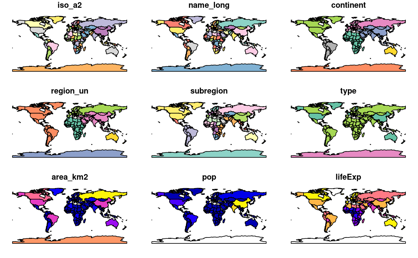

FIGURE 2.3: A spatial plot of the world using the sf package, with a facet for each attribute.

Note that instead of creating a single map, as most GIS programs would, the plot() command has created multiple maps, one for each variable in the world datasets. This behavior can be useful for exploring the spatial distribution of different variables and is discussed further in Section 2.2.3 below.

Being able to treat spatial objects as regular data frames with spatial powers has many advantages, especially if you are already used to working with data frames. The commonly used summary() function, for example, provides a useful overview of the variables within the world object.

summary(world["lifeExp"])
#>     lifeExp                geom    
#>  Min.   :50.6   MULTIPOLYGON :177  
#>  1st Qu.:65.0   epsg:4326    :  0  
#>  Median :72.9   +proj=long...:  0  
#>  Mean   :70.9                      
#>  3rd Qu.:76.8                      
#>  Max.   :83.6                      
#>  NA's   :10

Although we have only selected one variable for the summary command, it also outputs a report on the geometry. This demonstrates the ‘sticky’ behavior of the geometry columns of sf objects, meaning the geometry is kept unless the user deliberately removes them, as we’ll see in Section 3.2. The result provides a quick summary of both the non-spatial and spatial data contained in world: the mean average life expectancy is 71 years (ranging from less than 51 to more than 83 years with a median of 73 years) across all countries.

The word MULTIPOLYGON in the summary output above refers to the geometry type of features (countries) in the world object. This representation is necessary for countries with islands such as Indonesia and Greece. Other geometry types are described in Section 2.2.5.

It is worth taking a deeper look at the basic behavior and contents of this simple feature object, which can usefully be thought of as a ‘spatial data frame.’

sf objects are easy to subset. The code below shows its first two rows and three columns. The output shows two major differences compared with a regular data.frame: the inclusion of additional geographic data (geometry type, dimension, bbox and CRS information - epsg (SRID), proj4string), and the presence of a geometry column, here named geom:

world_mini = world[1:2, 1:3]
world_mini
#> Simple feature collection with 2 features and 3 fields
#> Geometry type: MULTIPOLYGON
#> Dimension:     XY
#> Bounding box:  xmin: -180 ymin: -18.3 xmax: 180 ymax: -0.95
#> Geodetic CRS:  WGS 84
#> # A tibble: 2 × 4
#>   iso_a2 name_long continent                                                geom
#>   <chr>  <chr>     <chr>                                      <MULTIPOLYGON [°]>
#> 1 FJ     Fiji      Oceania   (((-180 -16.6, -180 -16.5, -180 -16, -180 -16.1, -…
#> 2 TZ     Tanzania  Africa    (((33.9 -0.95, 31.9 -1.03, 30.8 -1.01, 30.4 -1.13,…

All this may seem rather complex, especially for a class system that is supposed to be simple. However, there are good reasons for organizing things this way and using sf.

Before describing each geometry type that the sf package supports, it is worth taking a step back to understand the building blocks of sf objects. Section 2.2.8 shows how simple features objects are data frames, with special geometry columns. These spatial columns are often called geom or geometry: world$geom refers to the spatial element of the world object described above. These geometry columns are ‘list columns’ of class sfc (see Section 2.2.7). In turn, sfc objects are composed of one or more objects of class sfg: simple feature geometries that we describe in Section 2.2.6.

To understand how the spatial components of simple features work, it is vital to understand simple feature geometries. For this reason we cover each currently supported simple features geometry type in Section 2.2.5 before moving on to describe how these can be represented in R using sfg objects, which form the basis of sfc and eventually full sf objects.

The preceding code chunk uses = to create a new object called world_mini in the command world_mini = world[1:2, 1:3]. This is called assignment. An equivalent command to achieve the same result is world_mini <- world[1:2, 1:3]. Although ‘arrow assigment’ is more commonly used, we use ‘equals assignment’ because it’s slightly faster to type and easier to teach due to compatibility with commonly used languages such as Python and JavaScript. Which to use is largely a matter of preference as long as you’re consistent (packages such as styler can be used to change style).

2.2.2 Why simple features?

Simple features is a widely supported data model that underlies data structures in many GIS applications including QGIS and PostGIS. A major advantage of this is that using the data model ensures your work is cross-transferable to other set-ups, for example importing from and exporting to spatial databases.

A more specific question from an R perspective is “why use the sf package when sp is already tried and tested?” There are many reasons (linked to the advantages of the simple features model):

• Fast reading and writing of data
• Enhanced plotting performance
• sf objects can be treated as data frames in most operations
• sf functions can be combined using %>% operator and works well with the tidyverse collection of R packages.
• sf function names are relatively consistent and intuitive (all begin with st_)

Due to such advantages, some spatial packages (including tmap, mapview and tidycensus) have added support for sf. However, it will take many years for most packages to transition and some will never switch. Fortunately, these can still be used in a workflow based on sf objects, by converting them to the Spatial class used in sp:

library(sp)
world_sp = as(world, Class = "Spatial")
# sp functions ...

Spatial objects can be converted back to sf in the same way or with st_as_sf():

world_sf = st_as_sf(world_sp)

2.2.3 Basic map making

Basic maps are created in sf with plot(). By default this creates a multi-panel plot (like sp’s spplot()), one sub-plot for each variable of the object, as illustrated in the left-hand panel in Figure 2.4. A legend or ‘key’ with a continuous color is produced if the object to be plotted has a single variable (see the right-hand panel). Colors can also be set with col =, although this will not create a continuous palette or a legend.

plot(world[3:6])
plot(world["pop"])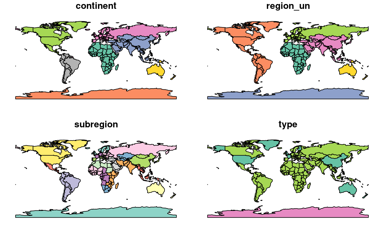

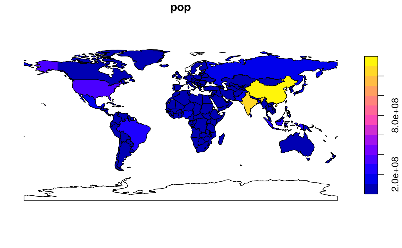
FIGURE 2.4: Plotting with sf, with multiple variables (left) and a single variable (right).

Plots are added as layers to existing images by setting add = TRUE.⁸ To demonstrate this, and to provide a taster of content covered in Chapters 3 and 4 on attribute and spatial data operations, the subsequent code chunk combines countries in Asia:

world_asia = world[world$continent == "Asia", ]
asia = st_union(world_asia)

We can now plot the Asian continent over a map of the world. Note that the first plot must only have one facet for add = TRUE to work. If the first plot has a key, reset = FALSE must be used (result not shown):

plot(world["pop"], reset = FALSE)
plot(asia, add = TRUE, col = "red")

Adding layers in this way can be used to verify the geographic correspondence between layers: the plot() function is fast to execute and requires few lines of code, but does not create interactive maps with a wide range of options. For more advanced map making we recommend using dedicated visualization packages such as tmap (see Chapter 8).

2.2.4 Base plot arguments

There are various ways to modify maps with sf’s plot() method. Because sf extends base R plotting methods plot()’s arguments such as main = (which specifies the title of the map) work with sf objects (see ?graphics::plot and ?par).⁹

Figure 2.5 illustrates this flexibility by overlaying circles, whose diameters (set with cex =) represent country populations, on a map of the world. An unprojected version of this figure can be created with the following commands (see exercises at the end of this chapter and the script 02-contplot.R to reproduce Figure 2.5):

plot(world["continent"], reset = FALSE)
cex = sqrt(world$pop) / 10000
world_cents = st_centroid(world, of_largest = TRUE)
plot(st_geometry(world_cents), add = TRUE, cex = cex)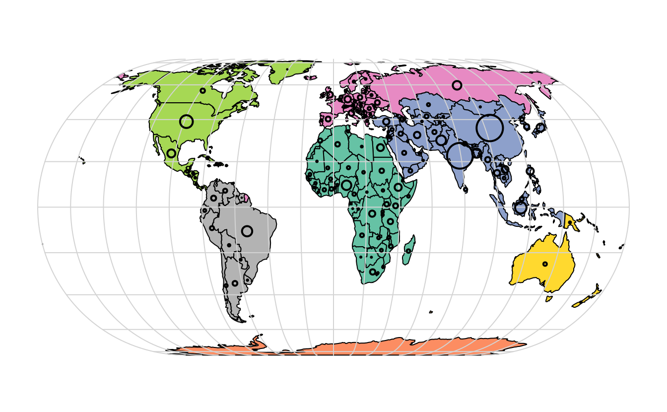

FIGURE 2.5: Country continents (represented by fill color) and 2015 populations (represented by circles, with area proportional to population).

The code above uses the function st_centroid() to convert one geometry type (polygons) to another (points) (see Chapter 5), the aesthetics of which are varied with the cex argument.

sf’s plot method also has arguments specific to geographic data. expandBB, for example, can be used to plot an sf object in context: it takes a numeric vector of length four that expands the bounding box of the plot relative to zero in the following order: bottom, left, top, right. This is used to plot India in the context of its giant Asian neighbors, with an emphasis on China to the east, in the following code chunk, which generates Figure 2.6 (see exercises below on adding text to plots):

india = world[world$name_long == "India", ]
plot(st_geometry(india), expandBB = c(0, 0.2, 0.1, 1), col = "gray", lwd = 3)
plot(world_asia[0], add = TRUE)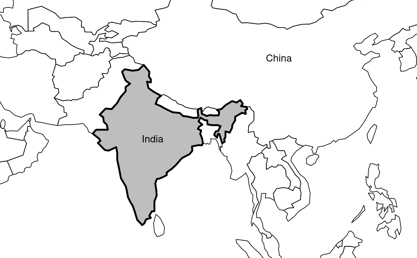

FIGURE 2.6: India in context, demonstrating the expandBB argument.

Note the use of [0] to keep only the geometry column and lwd to emphasize India. See Section 8.6 for other visualization techniques for representing a range of geometry types, the subject of the next section.

2.2.5 Geometry types

Geometries are the basic building blocks of simple features. Simple features in R can take on one of the 17 geometry types supported by the sf package. In this chapter we will focus on the seven most commonly used types: POINT, LINESTRING, POLYGON, MULTIPOINT, MULTILINESTRING, MULTIPOLYGON and GEOMETRYCOLLECTION. Find the whole list of possible feature types in the PostGIS manual.

Generally, well-known binary (WKB) or well-known text (WKT) are the standard encoding for simple feature geometries. WKB representations are usually hexadecimal strings easily readable for computers. This is why GIS and spatial databases use WKB to transfer and store geometry objects. WKT, on the other hand, is a human-readable text markup description of simple features. Both formats are exchangeable, and if we present one, we will naturally choose the WKT representation.

The basis for each geometry type is the point. A point is simply a coordinate in 2D, 3D or 4D space (see vignette("sf1") for more information) such as (see left panel in Figure 2.7):

• POINT (5 2)

A linestring is a sequence of points with a straight line connecting the points, for example (see middle panel in Figure 2.7):

• LINESTRING (1 5, 4 4, 4 1, 2 2, 3 2)

A polygon is a sequence of points that form a closed, non-intersecting ring. Closed means that the first and the last point of a polygon have the same coordinates (see right panel in Figure 2.7).¹⁰

• Polygon without a hole: POLYGON ((1 5, 2 2, 4 1, 4 4, 1 5))

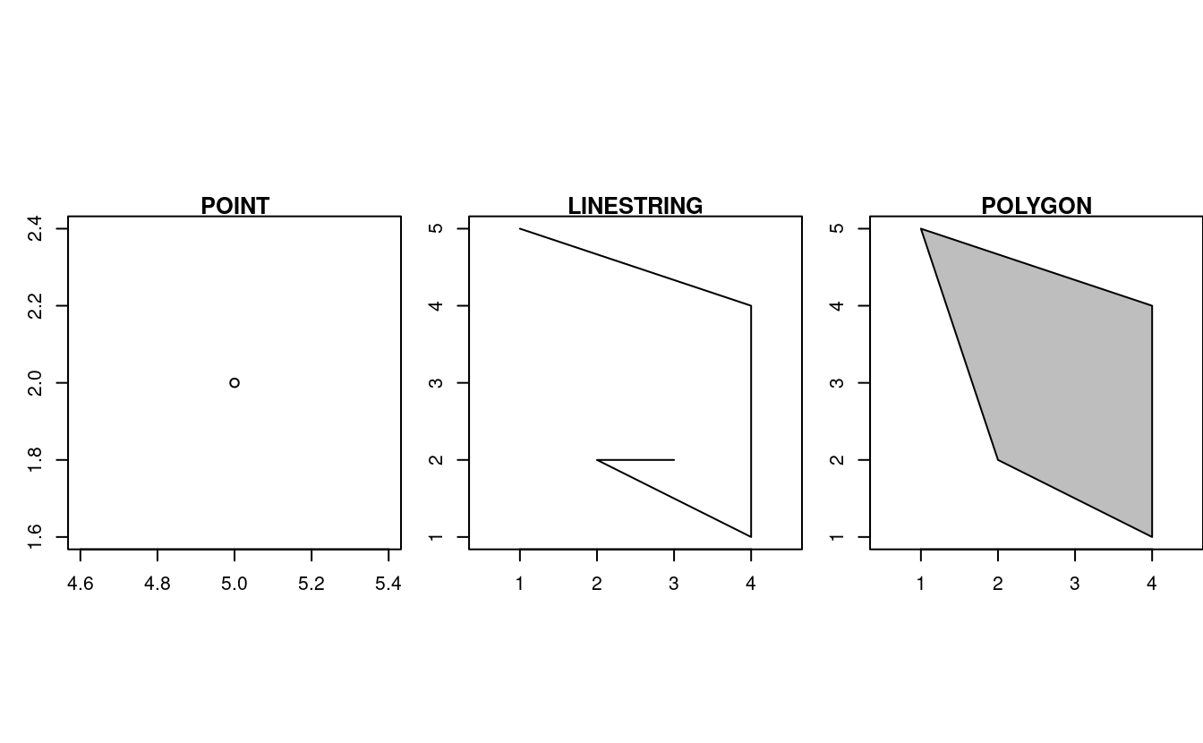
FIGURE 2.7: Illustration of point, linestring and polygon geometries.

So far we have created geometries with only one geometric entity per feature. However, sf also allows multiple geometries to exist within a single feature (hence the term ‘geometry collection’) using “multi” version of each geometry type:

• Multipoint: MULTIPOINT (5 2, 1 3, 3 4, 3 2)
• Multilinestring: MULTILINESTRING ((1 5, 4 4, 4 1, 2 2, 3 2), (1 2, 2 4))
• Multipolygon: MULTIPOLYGON (((1 5, 2 2, 4 1, 4 4, 1 5), (0 2, 1 2, 1 3, 0 3, 0 2)))

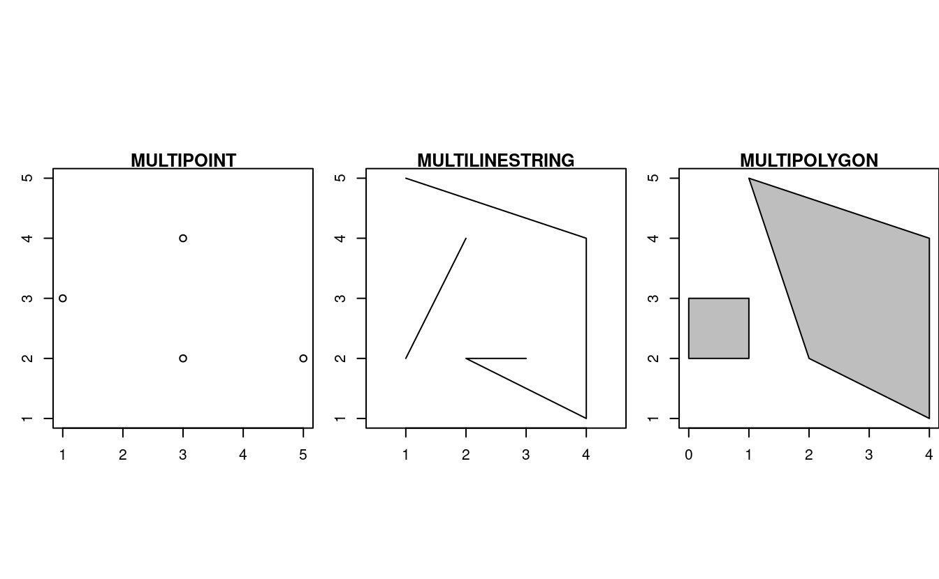
FIGURE 2.8: Illustration of multi* geometries.

Finally, a geometry collection can contain any combination of geometries including (multi)points and linestrings (see Figure 2.9):

• Geometry collection: GEOMETRYCOLLECTION (MULTIPOINT (5 2, 1 3, 3 4, 3 2), LINESTRING (1 5, 4 4, 4 1, 2 2, 3 2))

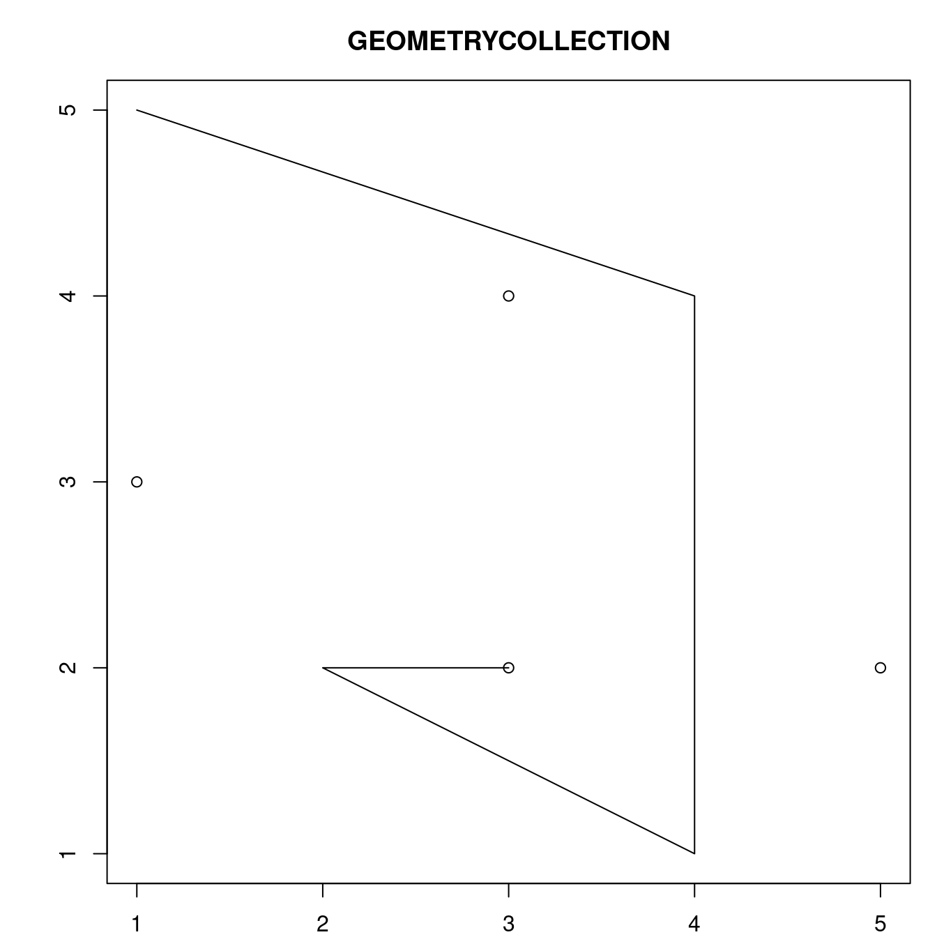
FIGURE 2.9: Illustration of a geometry collection.

2.2.6 Simple feature geometries (sfg)

The sfg class represents the different simple feature geometry types in R: point, linestring, polygon (and their ‘multi’ equivalents, such as multipoints) or geometry collection.

Usually you are spared the tedious task of creating geometries on your own since you can simply import an already existing spatial file. However, there are a set of functions to create simple feature geometry objects (sfg) from scratch if needed. The names of these functions are simple and consistent, as they all start with the st_ prefix and end with the name of the geometry type in lowercase letters:

• A point: st_point()
• A linestring: st_linestring()
• A polygon: st_polygon()
• A multipoint: st_multipoint()
• A multilinestring: st_multilinestring()
• A multipolygon: st_multipolygon()
• A geometry collection: st_geometrycollection()

sfg objects can be created from three base R data types:

1. A numeric vector: a single point
2. A matrix: a set of points, where each row represents a point, a multipoint or linestring
3. A list: a collection of objects such as matrices, multilinestrings or geometry collections

The function st_point() creates single points from numeric vectors:

st_point(c(5, 2))                 # XY point
#> POINT (5 2)
st_point(c(5, 2, 3))              # XYZ point
#> POINT Z (5 2 3)
st_point(c(5, 2, 1), dim = "XYM") # XYM point
#> POINT M (5 2 1)
st_point(c(5, 2, 3, 1))           # XYZM point
#> POINT ZM (5 2 3 1)

The results show that XY (2D coordinates), XYZ (3D coordinates) and XYZM (3D with an additional variable, typically measurement accuracy) point types are created from vectors of length 2, 3, and 4, respectively. The XYM type must be specified using the dim argument (which is short for dimension).

By contrast, use matrices in the case of multipoint (st_multipoint()) and linestring (st_linestring()) objects:

# the rbind function simplifies the creation of matrices
## MULTIPOINT
multipoint_matrix = rbind(c(5, 2), c(1, 3), c(3, 4), c(3, 2))
st_multipoint(multipoint_matrix)
#> MULTIPOINT ((5 2), (1 3), (3 4), (3 2))
## LINESTRING
linestring_matrix = rbind(c(1, 5), c(4, 4), c(4, 1), c(2, 2), c(3, 2))
st_linestring(linestring_matrix)
#> LINESTRING (1 5, 4 4, 4 1, 2 2, 3 2)

Finally, use lists for the creation of multilinestrings, (multi-)polygons and geometry collections:

## POLYGON
polygon_list = list(rbind(c(1, 5), c(2, 2), c(4, 1), c(4, 4), c(1, 5)))
st_polygon(polygon_list)
#> POLYGON ((1 5, 2 2, 4 1, 4 4, 1 5))

## POLYGON with a hole
polygon_border = rbind(c(1, 5), c(2, 2), c(4, 1), c(4, 4), c(1, 5))
polygon_hole = rbind(c(2, 4), c(3, 4), c(3, 3), c(2, 3), c(2, 4))
polygon_with_hole_list = list(polygon_border, polygon_hole)
st_polygon(polygon_with_hole_list)
#> POLYGON ((1 5, 2 2, 4 1, 4 4, 1 5), (2 4, 3 4, 3 3, 2 3, 2 4))

## MULTILINESTRING
multilinestring_list = list(rbind(c(1, 5), c(4, 4), c(4, 1), c(2, 2), c(3, 2)), 
                            rbind(c(1, 2), c(2, 4)))
st_multilinestring((multilinestring_list))
#> MULTILINESTRING ((1 5, 4 4, 4 1, 2 2, 3 2), (1 2, 2 4))

## MULTIPOLYGON
multipolygon_list = list(list(rbind(c(1, 5), c(2, 2), c(4, 1), c(4, 4), c(1, 5))),
                         list(rbind(c(0, 2), c(1, 2), c(1, 3), c(0, 3), c(0, 2))))
st_multipolygon(multipolygon_list)
#> MULTIPOLYGON (((1 5, 2 2, 4 1, 4 4, 1 5)), ((0 2, 1 2, 1 3, 0 3, 0 2)))

## GEOMETRYCOLLECTION
gemetrycollection_list = list(st_multipoint(multipoint_matrix),
                              st_linestring(linestring_matrix))
st_geometrycollection(gemetrycollection_list)
#> GEOMETRYCOLLECTION (MULTIPOINT (5 2, 1 3, 3 4, 3 2),
#>   LINESTRING (1 5, 4 4, 4 1, 2 2, 3 2))

2.2.7 Simple feature columns (sfc)

One sfg object contains only a single simple feature geometry. A simple feature geometry column (sfc) is a list of sfg objects, which is additionally able to contain information about the coordinate reference system in use. For instance, to combine two simple features into one object with two features, we can use the st_sfc() function. This is important since sfc represents the geometry column in sf data frames:

# sfc POINT
point1 = st_point(c(5, 2))
point2 = st_point(c(1, 3))
points_sfc = st_sfc(point1, point2)
points_sfc
#> Geometry set for 2 features 
#> Geometry type: POINT
#> Dimension:     XY
#> Bounding box:  xmin: 1 ymin: 2 xmax: 5 ymax: 3
#> CRS:           NA
#> POINT (5 2)
#> POINT (1 3)

In most cases, an sfc object contains objects of the same geometry type. Therefore, when we convert sfg objects of type polygon into a simple feature geometry column, we would also end up with an sfc object of type polygon, which can be verified with st_geometry_type(). Equally, a geometry column of multilinestrings would result in an sfc object of type multilinestring:

# sfc POLYGON
polygon_list1 = list(rbind(c(1, 5), c(2, 2), c(4, 1), c(4, 4), c(1, 5)))
polygon1 = st_polygon(polygon_list1)
polygon_list2 = list(rbind(c(0, 2), c(1, 2), c(1, 3), c(0, 3), c(0, 2)))
polygon2 = st_polygon(polygon_list2)
polygon_sfc = st_sfc(polygon1, polygon2)
st_geometry_type(polygon_sfc)
#> [1] POLYGON POLYGON
#> 18 Levels: GEOMETRY POINT LINESTRING POLYGON MULTIPOINT ... TRIANGLE

# sfc MULTILINESTRING
multilinestring_list1 = list(rbind(c(1, 5), c(4, 4), c(4, 1), c(2, 2), c(3, 2)), 
                            rbind(c(1, 2), c(2, 4)))
multilinestring1 = st_multilinestring((multilinestring_list1))
multilinestring_list2 = list(rbind(c(2, 9), c(7, 9), c(5, 6), c(4, 7), c(2, 7)), 
                            rbind(c(1, 7), c(3, 8)))
multilinestring2 = st_multilinestring((multilinestring_list2))
multilinestring_sfc = st_sfc(multilinestring1, multilinestring2)
st_geometry_type(multilinestring_sfc)
#> [1] MULTILINESTRING MULTILINESTRING
#> 18 Levels: GEOMETRY POINT LINESTRING POLYGON MULTIPOINT ... TRIANGLE

It is also possible to create an sfc object from sfg objects with different geometry types:

# sfc GEOMETRY
point_multilinestring_sfc = st_sfc(point1, multilinestring1)
st_geometry_type(point_multilinestring_sfc)
#> [1] POINT           MULTILINESTRING
#> 18 Levels: GEOMETRY POINT LINESTRING POLYGON MULTIPOINT ... TRIANGLE

As mentioned before, sfc objects can additionally store information on the coordinate reference systems (CRS). To specify a certain CRS, we can use the epsg (SRID) or proj4string attributes of an sfc object. The default value of epsg (SRID) and proj4string is NA (Not Available), as can be verified with st_crs():

st_crs(points_sfc)
#> Coordinate Reference System: NA

All geometries in an sfc object must have the same CRS. We can add coordinate reference system as a crs argument of st_sfc(). This argument accepts an integer with the epsg code such as 4326, which automatically adds the ‘proj4string’ (see Section 2.4):

# EPSG definition
points_sfc_wgs = st_sfc(point1, point2, crs = 4326)
st_crs(points_sfc_wgs)
#> Coordinate Reference System:
#>   User input: EPSG:4326 
#>   wkt:
#> GEOGCRS["WGS 84",
#>     DATUM["World Geodetic System 1984",
#>         ELLIPSOID["WGS 84",6378137,298.257223563,
#>             LENGTHUNIT["metre",1]]],
#>     PRIMEM["Greenwich",0,
#>         ANGLEUNIT["degree",0.0174532925199433]],
#>     CS[ellipsoidal,2],
#>         AXIS["geodetic latitude (Lat)",north,
#>             ORDER[1],
#>             ANGLEUNIT["degree",0.0174532925199433]],
#>         AXIS["geodetic longitude (Lon)",east,
#>             ORDER[2],
#>             ANGLEUNIT["degree",0.0174532925199433]],
#>     USAGE[
#>         SCOPE["Horizontal component of 3D system."],
#>         AREA["World."],
#>         BBOX[-90,-180,90,180]],
#>     ID["EPSG",4326]]

It also accepts a raw proj4string (result not shown):

# PROJ4STRING definition
st_sfc(point1, point2, crs = "+proj=longlat +datum=WGS84 +no_defs")

Sometimes st_crs() will return a proj4string but not an epsg code. This is because there is no general method to convert from proj4string to epsg (see Chapter 6).

2.2.8 The sf class

Sections 2.2.5 to 2.2.7 deal with purely geometric objects, ‘sf geometry’ and ‘sf column’ objects, respectively. These are geographic building blocks of geographic vector data represented as simple features. The final building block is non-geographic attributes, representing the name of the feature or other attributes such as measured values, groups, and other things.

To illustrate attributes, we will represent a temperature of 25°C in London on June 21^st, 2017. This example contains a geometry (the coordinates), and three attributes with three different classes (place name, temperature and date).¹¹ Objects of class sf represent such data by combining the attributes (data.frame) with the simple feature geometry column (sfc). They are created with st_sf() as illustrated below, which creates the London example described above:

lnd_point = st_point(c(0.1, 51.5))                 # sfg object
lnd_geom = st_sfc(lnd_point, crs = 4326)           # sfc object
lnd_attrib = data.frame(                           # data.frame object
  name = "London",
  temperature = 25,
  date = as.Date("2017-06-21")
  )
lnd_sf = st_sf(lnd_attrib, geometry = lnd_geom)    # sf object

What just happened? First, the coordinates were used to create the simple feature geometry (sfg). Second, the geometry was converted into a simple feature geometry column (sfc), with a CRS. Third, attributes were stored in a data.frame, which was combined with the sfc object with st_sf(). This results in an sf object, as demonstrated below (some output is omitted):

lnd_sf
#> Simple feature collection with 1 features and 3 fields
#> ...
#>     name temperature       date         geometry
#> 1 London          25 2017-06-21 POINT (0.1 51.5)

class(lnd_sf)
#> [1] "sf"         "data.frame"

The result shows that sf objects actually have two classes, sf and data.frame. Simple features are simply data frames (square tables), but with spatial attributes stored in a list column, usually called geometry, as described in Section 2.2.1. This duality is central to the concept of simple features: most of the time a sf can be treated as and behaves like a data.frame. Simple features are, in essence, data frames with a spatial extension.

2.3 Raster data

The geographic raster data model usually consists of a raster header and a matrix (with rows and columns) representing equally spaced cells (often also called pixels; Figure 2.10:A).¹² The raster header defines the coordinate reference system, the extent and the origin. The origin (or starting point) is frequently the coordinate of the lower-left corner of the matrix (the raster package, however, uses the upper left corner, by default (Figure 2.10:B)). The header defines the extent via the number of columns, the number of rows and the cell size resolution. Hence, starting from the origin, we can easily access and modify each single cell by either using the ID of a cell (Figure 2.10:B) or by explicitly specifying the rows and columns. This matrix representation avoids storing explicitly the coordinates for the four corner points (in fact it only stores one coordinate, namely the origin) of each cell corner as would be the case for rectangular vector polygons. This and map algebra makes raster processing much more efficient and faster than vector data processing. However, in contrast to vector data, the cell of one raster layer can only hold a single value. The value might be numeric or categorical (Figure 2.10:C).

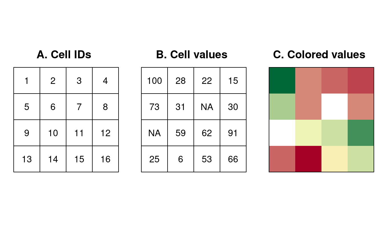
FIGURE 2.10: Raster data types: (A) cell IDs, (B) cell values, (C) a colored raster map.

Raster maps usually represent continuous phenomena such as elevation, temperature, population density or spectral data (Figure 2.11). Of course, we can represent discrete features such as soil or land-cover classes also with the help of a raster data model (Figure 2.11). Consequently, the discrete borders of these features become blurred, and depending on the spatial task a vector representation might be more suitable.

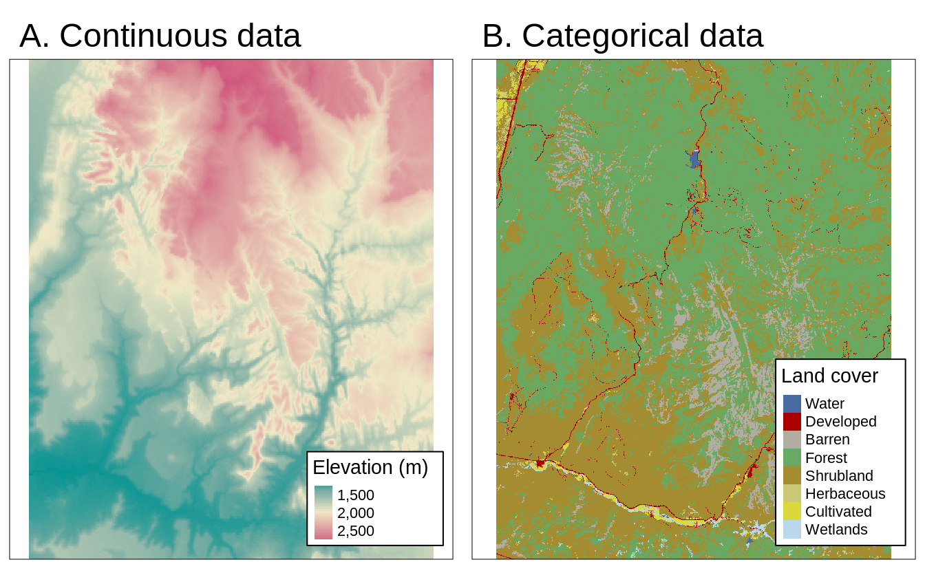
FIGURE 2.11: Examples of continuous and categorical rasters.

2.3.1 An introduction to raster

The raster package supports raster objects in R. It provides an extensive set of functions to create, read, export, manipulate and process raster datasets. Aside from general raster data manipulation, raster provides many low-level functions that can form the basis to develop more advanced raster functionality. raster also lets you work on large raster datasets that are too large to fit into the main memory. In this case, raster provides the possibility to divide the raster into smaller chunks (rows or blocks), and processes these iteratively instead of loading the whole raster file into RAM (for more information, please refer to vignette("functions", package = "raster").

For the illustration of raster concepts, we will use datasets from the spDataLarge (note these packages were loaded at the beginning of the chapter). It consists of a few raster objects and one vector object covering an area of the Zion National Park (Utah, USA). For example, srtm.tif is a digital elevation model of this area (for more details, see its documentation ?srtm). First, let’s create a RasterLayer object named new_raster:

raster_filepath = system.file("raster/srtm.tif", package = "spDataLarge")
new_raster = raster(raster_filepath)

Typing the name of the raster into the console, will print out the raster header (extent, dimensions, resolution, CRS) and some additional information (class, data source name, summary of the raster values):

new_raster
#> class       : RasterLayer 
#> dimensions  : 457, 465, 212505  (nrow, ncol, ncell)
#> resolution  : 0.000833, 0.000833  (x, y)
#> extent      : -113, -113, 37.1, 37.5  (xmin, xmax, ymin, ymax)
#> coord. ref. : +proj=longlat +datum=WGS84 +no_defs +ellps=WGS84 +towgs84=0,0,0 
#> data source : /home/robin/R/x86_64-pc-linux../3.5/spDataLarge/raster/srtm.tif 
#> names       : srtm 
#> values      : 1024, 2892  (min, max)

Dedicated functions report each component: dim(new_raster) returns the number of rows, columns and layers; the ncell() function the number of cells (pixels); res() the raster’s spatial resolution; extent() its spatial extent; and crs() its coordinate reference system (raster reprojection is covered in Section 6.6). inMemory() reports whether the raster data is stored in memory (the default) or on disk.

help("raster-package") returns a full list of all available raster functions.

2.3.2 Basic map making

Similar to the sf package, raster also provides plot() methods for its own classes.

plot(new_raster)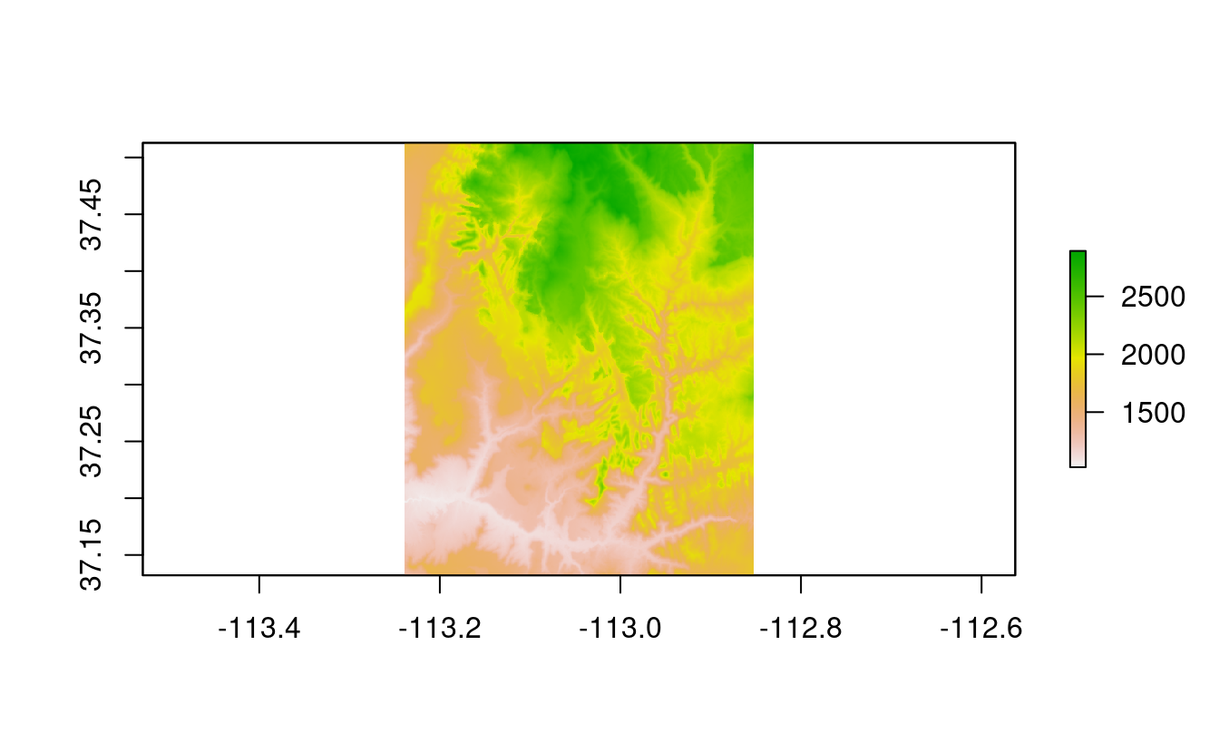

FIGURE 2.12: Basic raster plot.

There are several other approaches for plotting raster data in R that are outside the scope of this section, including:

• functions such as spplot() and levelplot() (from the sp and rasterVis packages, respectively) to create facets, a common technique for visualizing change over time; and
• packages such as tmap, mapview and leaflet to create interactive maps of raster and vector objects (see Chapter 8).

2.3.3 Raster classes

The RasterLayer class represents the simplest form of a raster object, and consists of only one layer. The easiest way to create a raster object in R is to read-in a raster file from disk or from a server.

raster_filepath = system.file("raster/srtm.tif", package = "spDataLarge")
new_raster = raster(raster_filepath)

The raster package supports numerous drivers with the help of rgdal. To find out which drivers are available on your system, run raster::writeFormats() and rgdal::gdalDrivers().

Rasters can also be created from scratch using the raster() function. This is illustrated in the subsequent code chunk, which results in a new RasterLayer object. The resulting raster consists of 36 cells (6 columns and 6 rows specified by nrows and ncols) centered around the Prime Meridian and the Equator (see xmn, xmx, ymn and ymx parameters). The CRS is the default of raster objects: WGS84. This means the unit of the resolution is in degrees which we set to 0.5 (res). Values (vals) are assigned to each cell: 1 to cell 1, 2 to cell 2, and so on. Remember: raster() fills cells row-wise (unlike matrix()) starting at the upper left corner, meaning the top row contains the values 1 to 6, the second 7 to 12, etc.

new_raster2 = raster(nrows = 6, ncols = 6, res = 0.5, 
                     xmn = -1.5, xmx = 1.5, ymn = -1.5, ymx = 1.5,
                     vals = 1:36)

For other ways of creating raster objects, see ?raster.

Aside from RasterLayer, there are two additional classes: RasterBrick and RasterStack. Both can handle multiple layers, but differ regarding the number of supported file formats, type of internal representation and processing speed.

A RasterBrick consists of multiple layers, which typically correspond to a single multispectral satellite file or a single multilayer object in memory. The brick() function creates a RasterBrick object. Usually, you provide it with a filename to a multilayer raster file but might also use another raster object and other spatial objects (see ?brick for all supported formats).

multi_raster_file = system.file("raster/landsat.tif", package = "spDataLarge")
r_brick = brick(multi_raster_file)

r_brick
#> class       : RasterBrick 
#> resolution  : 30, 30  (x, y)
#> ...
#> names       : landsat.1, landsat.2, landsat.3, landsat.4 
#> min values  :      7550,      6404,      5678,      5252 
#> max values  :     19071,     22051,     25780,     31961

nlayers() retrieves the number of layers stored in a Raster* object:

nlayers(r_brick)
#> [1] 4

A RasterStack is similar to a RasterBrick in the sense that it consists also of multiple layers. However, in contrast to RasterBrick, RasterStack allows you to connect several raster objects stored in different files or multiple objects in memory. More specifically, a RasterStack is a list of RasterLayer objects with the same extent and resolution. Hence, one way to create it is with the help of spatial objects already existing in R’s global environment. And again, one can simply specify a path to a file stored on disk.

raster_on_disk = raster(r_brick, layer = 1)
raster_in_memory = raster(xmn = 301905, xmx = 335745,
                          ymn = 4111245, ymx = 4154085, 
                          res = 30)
values(raster_in_memory) = sample(seq_len(ncell(raster_in_memory)))
crs(raster_in_memory) = crs(raster_on_disk)

r_stack = stack(raster_in_memory, raster_on_disk)
r_stack
#> class : RasterStack
#> dimensions : 1428, 1128, 1610784, 2
#> resolution : 30, 30
#> ...
#> names       :   layer, landsat.1 
#> min values  :       1,      7550 
#> max values  : 1610784,     19071

Another difference is that the processing time for RasterBrick objects is usually shorter than for RasterStack objects.

Decision on which Raster* class should be used depends mostly on the character of input data. Processing of a single mulitilayer file or object is the most effective with RasterBrick, while RasterStack allows calculations based on many files, many Raster* objects, or both.

Operations on RasterBrick and RasterStack objects will typically return a RasterBrick.

2.4 Coordinate Reference Systems

Vector and raster spatial data types share concepts intrinsic to spatial data. Perhaps the most fundamental of these is the Coordinate Reference System (CRS), which defines how the spatial elements of the data relate to the surface of the Earth (or other bodies). CRSs are either geographic or projected, as introduced at the beginning of this chapter (see Figure 2.1). This section will explain each type, laying the foundations for Section 6 on CRS transformations.

2.4.1 Geographic coordinate systems

Geographic coordinate systems identify any location on the Earth’s surface using two values — longitude and latitude (see left panels of Figures 2.13 and 2.14). Longitude is location in the East-West direction in angular distance from the Prime Meridian plane. Latitude is angular distance North or South of the equatorial plane. Distances in geographic CRSs are therefore not measured in meters. This has important consequences, as demonstrated in Section 6.

The surface of the Earth in geographic coordinate systems is represented by a spherical or ellipsoidal surface. Spherical models assume that the Earth is a perfect sphere of a given radius. Spherical models have the advantage of simplicity but are rarely used because they are inaccurate: the Earth is not a sphere! Ellipsoidal models are defined by two parameters: the equatorial radius and the polar radius. These are suitable because the Earth is compressed: the equatorial radius is around 11.5 km longer than the polar radius (Maling 1992).¹³

Ellipsoids are part of a wider component of CRSs: the datum. This contains information on what ellipsoid to use (with the ellps parameter in the PROJ CRS library) and the precise relationship between the Cartesian coordinates and location on the Earth’s surface. These additional details are stored in the towgs84 argument of proj4string notation (see proj.org/usage/projections.html for details). These allow local variations in Earth’s surface, for example due to large mountain ranges, to be accounted for in a local CRS. There are two types of datum — local and geocentric. In a local datum such as NAD83 the ellipsoidal surface is shifted to align with the surface at a particular location. In a geocentric datum such as WGS84 the center is the Earth’s center of gravity and the accuracy of projections is not optimized for a specific location.

2.4.2 Projected coordinate reference systems

Projected CRSs are based on Cartesian coordinates on an implicitly flat surface (right panels of Figures 2.13 and 2.14). They have an origin, x and y axes, and a linear unit of measurement such as meters. All projected CRSs are based on a geographic CRS, described in the previous section, and rely on map projections to convert the three-dimensional surface of the Earth into Easting and Northing (x and y) values in a projected CRS.

This transition cannot be done without adding some distortion. Therefore, some properties of the Earth’s surface are distorted in this process, such as area, direction, distance, and shape. A projected coordinate system can preserve only one or two of those properties. Projections are often named based on a property they preserve: equal-area preserves area, azimuthal preserve direction, equidistant preserve distance, and conformal preserve local shape.

There are three main groups of projection types - conic, cylindrical, and planar. In a conic projection, the Earth’s surface is projected onto a cone along a single line of tangency or two lines of tangency. Distortions are minimized along the tangency lines and rise with the distance from those lines in this projection. Therefore, it is the best suited for maps of mid-latitude areas. A cylindrical projection maps the surface onto a cylinder. This projection could also be created by touching the Earth’s surface along a single line of tangency or two lines of tangency. Cylindrical projections are used most often when mapping the entire world. A planar projection projects data onto a flat surface touching the globe at a point or along a line of tangency. It is typically used in mapping polar regions. st_proj_info(type = "proj") gives a list of the available projections supported by the PROJ library.

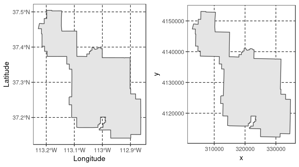
FIGURE 2.13: Examples of geographic (WGS 84; left) and projected (NAD83 / UTM zone 12N; right) coordinate systems for a vector data type.

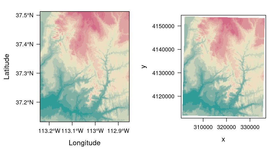
FIGURE 2.14: Examples of geographic (WGS 84; left) and projected (NAD83 / UTM zone 12N; right) coordinate systems for raster data.

2.4.3 CRSs in R

Two main ways to describe CRS in R are an epsg code or a proj4string definition. Both of these approaches have advantages and disadvantages. An epsg code is usually shorter, and therefore easier to remember. The code also refers to only one, well-defined coordinate reference system. On the other hand, a proj4string definition allows you more flexibility when it comes to specifying different parameters such as the projection type, the datum and the ellipsoid.¹⁴ This way you can specify many different projections, and modify existing ones. This also makes the proj4string approach more complicated. epsg points to exactly one particular CRS.

Spatial R packages support a wide range of CRSs and they use the long-established PROJ library. Other than searching for EPSG codes online, another quick way to find out about available CRSs is via the rgdal::make_EPSG() function, which outputs a data frame of available projections. Before going into more detail, it’s worth learning how to view and filter them inside R, as this could save time trawling the internet. The following code will show available CRSs interactively, allowing you to filter ones of interest (try filtering for the OSGB CRSs for example):

crs_data = rgdal::make_EPSG()
View(crs_data)

In sf the CRS of an object can be retrieved using st_crs(). For this, we need to read-in a vector dataset:

vector_filepath = system.file("vector/zion.gpkg", package = "spDataLarge")
new_vector = st_read(vector_filepath)

Our new object, new_vector, is a polygon representing the borders of Zion National Park (?zion).

st_crs(new_vector) # get CRS
#> Coordinate Reference System:
#> No EPSG code
#> proj4string: "+proj=utm +zone=12 +ellps=GRS80 ... +units=m +no_defs"

In cases when a coordinate reference system (CRS) is missing or the wrong CRS is set, the st_set_crs() function can be used:

new_vector = st_set_crs(new_vector, 4326) # set CRS
#> Warning: st_crs<- : replacing crs does not reproject data; use st_transform for
#> that

The warning message informs us that the st_set_crs() function does not transform data from one CRS to another.

The projection() function can be used to access CRS information from a Raster* object:

projection(new_raster) # get CRS
#> [1] "+proj=longlat +datum=WGS84 +no_defs"

The same function, projection(), is used to set a CRS for raster objects. The main difference, compared to vector data, is that raster objects only accept proj4 definitions:

new_raster3 = new_raster
projection(new_raster3) = "+proj=utm +zone=12 +ellps=GRS80 +towgs84=0,0,0,0,0,0,0 
                            +units=m +no_defs" # set CRS

Importantly, the st_crs() and projection() functions do not alter coordinates’ values or geometries. Their role is only to set a metadata information about the object CRS. We will expand on CRSs and explain how to project from one CRS to another in Chapter 6.

2.5 Units

An important feature of CRSs is that they contain information about spatial units. Clearly, it is vital to know whether a house’s measurements are in feet or meters, and the same applies to maps. It is good cartographic practice to add a scale bar onto maps to demonstrate the relationship between distances on the page or screen and distances on the ground. Likewise, it is important to formally specify the units in which the geometry data or pixels are measured to provide context, and ensure that subsequent calculations are done in context.

A novel feature of geometry data in sf objects is that they have native support for units. This means that distance, area and other geometric calculations in sf return values that come with a units attribute, defined by the units package (E. Pebesma, Mailund, and Hiebert 2016). This is advantageous, preventing confusion caused by different units (most CRSs use meters, some use feet) and providing information on dimensionality. This is demonstrated in the code chunk below, which calculates the area of Luxembourg:

luxembourg = world[world$name_long == "Luxembourg", ]

st_area(luxembourg) # requires the s2 package in recent versions of sf
#> 2.41e+09 [m^2]

The output is in units of square meters (m²), showing that the result represents two-dimensional space. This information, stored as an attribute (which interested readers can discover with attributes(st_area(luxembourg))), can feed into subsequent calculations that use units, such as population density (which is measured in people per unit area, typically per km²). Reporting units prevents confusion. To take the Luxembourg example, if the units remained unspecified, one could incorrectly assume that the units were in hectares. To translate the huge number into a more digestible size, it is tempting to divide the results by a million (the number of square meters in a square kilometer):

st_area(luxembourg) / 1000000
#> 2409 [m^2]

However, the result is incorrectly given again as square meters. The solution is to set the correct units with the units package:

units::set_units(st_area(luxembourg), km^2)
#> 2409 [km^2]

Units are of equal importance in the case of raster data. However, so far sf is the only spatial package that supports units, meaning that people working on raster data should approach changes in the units of analysis (for example, converting pixel widths from imperial to decimal units) with care. The new_raster object (see above) uses a WGS84 projection with decimal degrees as units. Consequently, its resolution is also given in decimal degrees but you have to know it, since the res() function simply returns a numeric vector.

res(new_raster)
#> [1] 0.000833 0.000833

If we used the UTM projection, the units would change.

repr = projectRaster(new_raster, crs = 26912)
res(repr)
#> [1] 73.8 92.5

Again, the res() command gives back a numeric vector without any unit, forcing us to know that the unit of the UTM projection is meters.

2.6 Exercises

1. Use summary() on the geometry column of the world data object. What does the output tell us about:
   • Its geometry type?
   • The number of countries?
   • Its coordinate reference system (CRS)?
2. Run the code that ‘generated’ the map of the world in Figure 2.5 at the end of Section 2.2.4. Find two similarities and two differences between the image on your computer and that in the book.
   • What does the cex argument do (see ?plot)?
   • Why was cex set to the sqrt(world$pop) / 10000?
   • Bonus: experiment with different ways to visualize the global population.
3. Use plot() to create maps of Nigeria in context (see Section 2.2.4).
   • Adjust the lwd, col and expandBB arguments of plot().
   • Challenge: read the documentation of text() and annotate the map.
4. Create an empty RasterLayer object called my_raster with 10 columns and 10 rows. Assign random values between 0 and 10 to the new raster and plot it.
5. Read-in the raster/nlcd2011.tif file from the spDataLarge package. What kind of information can you get about the properties of this file?

Reminder: solutions can be found online at https://geocompr.github.io

References

Bivand, Roger, Tim Keitt, and Barry Rowlingson. 2018. Rgdal: Bindings for the ’Geospatial’ Data Abstraction Library. https://CRAN.R-project.org/package=rgdal.

Bivand, Roger, and Colin Rundel. 2018. Rgeos: Interface to Geometry Engine - Open Source (’GEOS’). https://CRAN.R-project.org/package=rgeos.

Gillespie, Colin, and Robin Lovelace. 2016. Efficient R Programming: A Practical Guide to Smarter Programming. O’Reilly Media.

Grolemund, Garrett, and Hadley Wickham. 2016. R for Data Science. O’Reilly Media.

Maling, D. H. 1992. Coordinate Systems and Map Projections. Second. Oxford ; New York: Pergamon Press.

Pebesma, Edzer. 2018. “Simple Features for R: Standardized Support for Spatial Vector Data.” The R Journal.

Pebesma, Edzer, and Roger Bivand. 2018. Sp: Classes and Methods for Spatial Data. https://CRAN.R-project.org/package=sp.

Pebesma, Edzer, Thomas Mailund, and James Hiebert. 2016. “Measurement Units in R.” The R Journal 8 (2): 486–94.

---

5. spDataLarge is not on CRAN, meaning it must be installed via remotes or with the following command: install.packages("spDataLarge", repos = "https://nowosad.github.io/drat/", type = "source"). ↩︎

6. The origin we are referring to, depicted in blue in Figure 2.1, is in fact the ‘false’ origin. The ‘true’ origin, the location at which distortions are at a minimum, is located at 2° W and 49° N. This was selected by the Ordnance Survey to be roughly in the center of the British landmass longitudinally. ↩︎

7. The full OGC standard includes rather exotic geometry types including ‘surface’ and ‘curve’ geometry types, which currently have limited application in real world applications. All 17 types can be represented with the sf package, although (as of summer 2018) plotting only works for the ‘core 7.’↩︎

8. plot()ing of sf objects uses sf:::plot.sf() behind the scenes. plot() is a generic method that behaves differently depending on the class of object being plotted.↩︎

9. Note: many plot arguments are ignored in facet maps, when more than one sf column is plotted.↩︎

10. By definition, a polygon has one exterior boundary (outer ring) and can have zero or more interior boundaries (inner rings), also known as holes. A polygon with a hole would be, for example, POLYGON ((1 5, 2 2, 4 1, 4 4, 1 5), (2 4, 3 4, 3 3, 2 3, 2 4))↩︎

11. Other attributes might include an urbanity category (city or village), or a remark if the measurement was made using an automatic station.↩︎

12. Depending on the file format the header is part of the actual image data file, e.g., GeoTIFF, or stored in an extra header or world file, e.g., ASCII grid formats. There is also the headerless (flat) binary raster format which should facilitate the import into various software programs. ↩︎

13. The degree of compression is often referred to as flattening, defined in terms of the equatorial radius (\(a\)) and polar radius (\(b\)) as follows: \(f = (a - b) / a\). The terms ellipticity and compression can also be used. Because \(f\) is a rather small value, digital ellipsoid models use the ‘inverse flattening’ (\(rf = 1/f\)) to define the Earth’s compression. Values of \(a\) and \(rf\) in various ellipsoidal models can be seen by executing sf_proj_info(type = "ellps").↩︎

14. A complete list of the proj4string parameters can be found at https://proj.org.↩︎