Chapter 3 Attribute data operations
Note: this is the first edition of Geocomputation with R, first published in 2019 and with minor updates since then until summer 2021. For the Second Edition of Geocomputation with R, due for publication in 2022, see geocompr.robinlovelace.net.
Prerequisites
- This chapter requires the following packages to be installed and attached:
library(sf)
library(raster)
library(dplyr)
library(stringr) # for working with strings (pattern matching)
library(tidyr) # for unite() and separate()- It also relies on spData, which loads datasets used in the code examples of this chapter:
library(spData)3.1 Introduction
Attribute data is non-spatial information associated with geographic (geometry) data. A bus stop provides a simple example: its position would typically be represented by latitude and longitude coordinates (geometry data), in addition to its name. The name is an attribute of the feature (to use Simple Features terminology) that bears no relation to its geometry.
Another example is the elevation value (attribute) for a specific grid cell in raster data. Unlike the vector data model, the raster data model stores the coordinate of the grid cell indirectly, meaning the distinction between attribute and spatial information is less clear. To illustrate the point, think of a pixel in the 3rd row and the 4th column of a raster matrix. Its spatial location is defined by its index in the matrix: move from the origin four cells in the x direction (typically east and right on maps) and three cells in the y direction (typically south and down). The raster’s resolution defines the distance for each x- and y-step which is specified in a header. The header is a vital component of raster datasets which specifies how pixels relate to geographic coordinates (see also Chapter 4).
The focus of this chapter is manipulating geographic objects based on attributes such as the name of a bus stop and elevation.
For vector data, this means operations such as subsetting and aggregation (see Sections 3.2.1 and 3.2.2).
These non-spatial operations have spatial equivalents:
the [ operator in base R, for example, works equally for subsetting objects based on their attribute and spatial objects, as we will see in Chapter 4.
This is good news: skills developed here are cross-transferable, meaning that this chapter lays the foundation for Chapter 4, which extends the methods presented here to the spatial world.
Sections 3.2.3 and 3.2.4 demonstrate how to join data onto simple feature objects using a shared ID and how to create new variables, respectively.
Raster attribute data operations are covered in Section 3.3, which covers creating continuous and categorical raster layers and extracting cell values from one layer and multiple layers (raster subsetting). Section 3.3.2 provides an overview of ‘global’ raster operations which can be used to characterize entire raster datasets.
3.2 Vector attribute manipulation
Geographic vector data in R are well supported by sf, a class which extends the data.frame.
Thus sf objects have one column per attribute variable (such as ‘name’) and one row per observation, or feature (e.g., per bus station).
sf objects also have a special column to contain geometry data, usually named geometry.
The geometry column is special because it is a list column, which can contain multiple geographic entities (points, lines, polygons) per row.
This was described in Chapter 2, which demonstrated how generic methods such as plot() and summary() work on sf objects.
sf also provides methods that allow sf objects to behave like regular data frames, as illustrated by other sf-specific methods that were originally developed for data frames:
methods(class = "sf") # methods for sf objects, first 12 shown#> [1] aggregate cbind coerce
#> [4] initialize merge plot
#> [7] print rbind [
#> [10] [[<- $<- show Many of these functions, including rbind() (for binding rows of data together) and $<- (for creating new columns) were developed for data frames.
A key feature of sf objects is that they store spatial and non-spatial data in the same way, as columns in a data.frame.
The geometry column of sf objects is typically called geometry but any name can be used.
The following command, for example, creates a geometry column named g:
st_sf(data.frame(n = world$name_long), g = world$geom)
wkb_geometry and the_geom.
sf objects also support tibble and tbl classes used in the tidyverse, allowing ‘tidy’ data analysis workflows for spatial data.
Thus sf enables the full power of R’s data analysis capabilities to be unleashed on geographic data.
Before using these capabilities it is worth re-capping how to discover the basic properties of vector data objects.
Let’s start by using base R functions to get a measure of the world dataset:
dim(world) # it is a 2 dimensional object, with rows and columns
#> [1] 177  11
nrow(world) # how many rows?
#> [1] 177
ncol(world) # how many columns?
#> [1] 11
Our dataset contains ten non-geographic columns (and one geometry list column) with almost 200 rows representing the world’s countries.
Extracting the attribute data of an sf object is the same as removing its geometry:
world_df = st_drop_geometry(world)
class(world_df)
#> [1] "tbl_df"     "tbl"        "data.frame"
This can be useful if the geometry column causes problems, e.g., by occupying large amounts of RAM, or to focus the attention on the attribute data.
For most cases, however, there is no harm in keeping the geometry column because non-spatial data operations on sf objects only change an object’s geometry when appropriate (e.g., by dissolving borders between adjacent polygons following aggregation).
This means that proficiency with attribute data in sf objects equates to proficiency with data frames in R.
For many applications, the tidyverse package dplyr offers the most effective and intuitive approach for working with data frames.
Tidyverse compatibility is an advantage of sf over its predecessor sp, but there are some pitfalls to avoid (see the supplementary tidyverse-pitfalls vignette at geocompr.github.io for details).
3.2.1 Vector attribute subsetting
Base R subsetting functions include [, subset() and $.
dplyr subsetting functions include select(), filter(), and pull().
Both sets of functions preserve the spatial components of attribute data in sf objects.
The [ operator can subset both rows and columns.
You use indices to specify the elements you wish to extract from an object, e.g., object[i, j], with i and j typically being numbers or logical vectors — TRUEs and FALSEs — representing rows and columns (they can also be character strings, indicating row or column names).
Leaving i or j empty returns all rows or columns, so world[1:5, ] returns the first five rows and all columns.
The examples below demonstrate subsetting with base R.
The results are not shown; check the results on your own computer:
world[1:6, ] # subset rows by position
world[, 1:3] # subset columns by position
world[, c("name_long", "lifeExp")] # subset columns by name
A demonstration of the utility of using logical vectors for subsetting is shown in the code chunk below.
This creates a new object, small_countries, containing nations whose surface area is smaller than 10,000 km2:
sel_area = world$area_km2 < 10000
summary(sel_area) # a logical vector
#>    Mode   FALSE    TRUE
#> logical     170       7
small_countries = world[sel_area, ]
The intermediary sel_area is a logical vector that shows that only seven countries match the query.
A more concise command, which omits the intermediary object, generates the same result:
small_countries = world[world$area_km2 < 10000, ]The base R function subset() provides yet another way to achieve the same result:
small_countries = subset(world, area_km2 < 10000)Base R functions are mature and widely used.
However, the more recent dplyr approach has several advantages.
It enables intuitive workflows.
It is fast, due to its C++ backend.
This is especially useful when working with big data as well as dplyr’s database integration.
The main dplyr subsetting functions are select(), slice(), filter() and pull().
raster and dplyr packages have a function called select(). When using both packages, the function in the most recently attached package will be used, ‘masking’ the incumbent function. This can generate error messages containing text like: unable to find an inherited method for function ‘select’ for signature ‘“sf”’. To avoid this error message, and prevent ambiguity, we use the long-form function name, prefixed by the package name and two colons (usually omitted from R scripts for concise code): dplyr::select().
select() selects columns by name or position.
For example, you could select only two columns, name_long and pop, with the following command (note the sticky geom column remains):
world1 = dplyr::select(world, name_long, pop)
names(world1)
#> [1] "name_long" "pop"       "geom"
select() also allows subsetting of a range of columns with the help of the : operator:
# all columns between name_long and pop (inclusive)
world2 = dplyr::select(world, name_long:pop)
Omit specific columns with the - operator:
# all columns except subregion and area_km2 (inclusive)
world3 = dplyr::select(world, -subregion, -area_km2)
Conveniently, select() lets you subset and rename columns at the same time, for example:
world4 = dplyr::select(world, name_long, population = pop)
names(world4)
#> [1] "name_long"  "population" "geom"
This is more concise than the base R equivalent:
world5 = world[, c("name_long", "pop")] # subset columns by name
names(world5)[names(world5) == "pop"] = "population" # rename column manually
select() also works with ‘helper functions’ for advanced subsetting operations, including contains(), starts_with() and num_range() (see the help page with ?select for details).
Most dplyr verbs return a data frame.
To extract a single vector, one has to explicitly use the pull() command.
The subsetting operator in base R (see ?[), by contrast, tries to return objects in the lowest possible dimension.
This means selecting a single column returns a vector in base R.
To turn off this behavior, set the drop argument to FALSE.
# create throw-away data frame
d = data.frame(pop = 1:10, area = 1:10)
# return data frame object when selecting a single column
d[, "pop", drop = FALSE] # equivalent to d["pop"]
select(d, pop)
# return a vector when selecting a single column
d[, "pop"]
pull(d, pop)
Due to the sticky geometry column, selecting a single attribute from an sf-object with the help of [() returns also a data frame.
Contrastingly, pull() and $ will give back a vector.
# data frame object
world[, "pop"]
# vector objects
world$pop
pull(world, pop)
slice() is the row-equivalent of select().
The following code chunk, for example, selects the 3rd to 5th rows:
slice(world, 3:5)filter() is dplyr’s equivalent of base R’s subset() function.
It keeps only rows matching given criteria, e.g., only countries with a very high average of life expectancy:
# Countries with a life expectancy longer than 82 years
world6 = filter(world, lifeExp > 82)
The standard set of comparison operators can be used in the filter() function, as illustrated in Table 3.1:
| Symbol | Name |
|---|---|
== |
Equal to |
!= |
Not equal to |
>, < |
Greater/Less than |
>=, <= |
Greater/Less than or equal |
&, |, ! |
Logical operators: And, Or, Not |
dplyr works well with the ‘pipe’ operator %>%, which takes its name from the Unix pipe | (Grolemund and Wickham 2016).
It enables expressive code: the output of a previous function becomes the first argument of the next function, enabling chaining.
This is illustrated below, in which only countries from Asia are filtered from the world dataset, next the object is subset by columns (name_long and continent) and the first five rows (result not shown).
world7 = world %>%
  filter(continent == "Asia") %>%
  dplyr::select(name_long, continent) %>%
  slice(1:5)
The above chunk shows how the pipe operator allows commands to be written in a clear order:
the above run from top to bottom (line-by-line) and left to right.
The alternative to %>% is nested function calls, which is harder to read:
world8 = slice(
  dplyr::select(
    filter(world, continent == "Asia"),
    name_long, continent),
  1:5)
3.2.2 Vector attribute aggregation
Aggregation operations summarize datasets by a ‘grouping variable,’ typically an attribute column (spatial aggregation is covered in the next chapter).
An example of attribute aggregation is calculating the number of people per continent based on country-level data (one row per country).
The world dataset contains the necessary ingredients: the columns pop and continent, the population and the grouping variable, respectively.
The aim is to find the sum() of country populations for each continent.
This can be done with the base R function aggregate() as follows:
world_agg1 = aggregate(pop ~ continent, FUN = sum, data = world, na.rm = TRUE)
class(world_agg1)
#> [1] "data.frame"
The result is a non-spatial data frame with six rows, one per continent, and two columns reporting the name and population of each continent (see Table 3.2 with results for the top 3 most populous continents).
aggregate() is a generic function which means that it behaves differently depending on its inputs.
sf provides the method aggregate.sf() which is activated automatically when x is an sf object and a by argument is provided:
world_agg2 = aggregate(world["pop"], by = list(world$continent),
                       FUN = sum, na.rm = TRUE)
class(world_agg2)
#> [1] "sf"         "data.frame"
As illustrated above, an object of class sf is returned this time.
world_agg2 which is a spatial object containing 6 polygons representing the continents of the world.
summarize() is the dplyr equivalent of aggregate().
It usually follows group_by(), which specifies the grouping variable, as illustrated below:
world_agg3 = world %>%
  group_by(continent) %>%
  summarize(pop = sum(pop, na.rm = TRUE))
This approach is flexible and gives control over the new column names. This is illustrated below: the command calculates the Earth’s population (~7 billion) and number of countries (result not shown):
world %>%
  summarize(pop = sum(pop, na.rm = TRUE), n = n())
In the previous code chunk pop and n are column names in the result.
sum() and n() were the aggregating functions.
The result is an sf object with a single row representing the world (this works thanks to the geometric operation ‘union,’ as explained in Section 5.2.6).
Let’s combine what we have learned so far about dplyr by chaining together functions to find the world’s 3 most populous continents (with dplyr::top_n()) and the number of countries they contain.
We can order the continents (rows) by decreasing population size for easier readability with dplyr::arrange() (the result of this command is presented in Table 3.2):
world %>%
  dplyr::select(pop, continent) %>%
  group_by(continent) %>%
  summarize(pop = sum(pop, na.rm = TRUE), n_countries = n()) %>%
  top_n(n = 3, wt = pop) %>%
  arrange(desc(pop)) %>%
st_drop_geometry()| continent | pop | n_countries |
|---|---|---|
| Asia | 4311408059 | 47 |
| Africa | 1154946633 | 51 |
| Europe | 669036256 | 39 |
?summarize and vignette(package = "dplyr") and Chapter 5 of R for Data Science.
3.2.3 Vector attribute joining
Combining data from different sources is a common task in data preparation.
Joins do this by combining tables based on a shared ‘key’ variable.
dplyr has multiple join functions including left_join() and inner_join() — see vignette("two-table") for a full list.
These function names follow conventions used in the database language SQL (Grolemund and Wickham 2016, chap. 13); using them to join non-spatial datasets to sf objects is the focus of this section.
dplyr join functions work the same on data frames and sf objects, the only important difference being the geometry list column.
The result of data joins can be either an sf or data.frame object.
The most common type of attribute join on spatial data takes an sf object as the first argument and adds columns to it from a data.frame specified as the second argument.
To demonstrate joins, we will combine data on coffee production with the world dataset.
The coffee data is in a data frame called coffee_data from the spData package (see ?coffee_data for details).
It has 3 columns:
name_long names major coffee-producing nations and coffee_production_2016 and coffee_production_2017 contain estimated values for coffee production in units of 60-kg bags in each year.
A ‘left join,’ which preserves the first dataset, merges world with coffee_data:
world_coffee = left_join(world, coffee_data)
#> Joining, by = "name_long"
class(world_coffee)
#> [1] "sf"         "tbl_df"     "tbl"        "data.frame"
Because the input datasets share a ‘key variable’ (name_long) the join worked without using the by argument (see ?left_join for details).
The result is an sf object identical to the original world object but with two new variables (with column indices 11 and 12) on coffee production.
This can be plotted as a map, as illustrated in Figure 3.1, generated with the plot() function below:
names(world_coffee)
#>  [1] "iso_a2"                 "name_long"              "continent"
#>  [4] "region_un"              "subregion"              "type"
#>  [7] "area_km2"               "pop"                    "lifeExp"
#> [10] "gdpPercap"              "geom"                   "coffee_production_2016"
#> [13] "coffee_production_2017"
plot(world_coffee["coffee_production_2017"])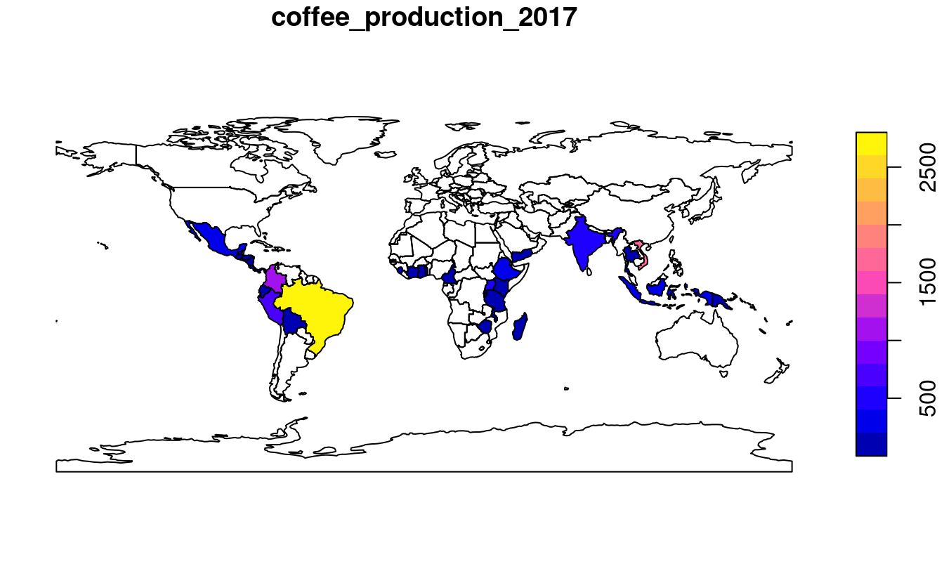
FIGURE 3.1: World coffee production (thousand 60-kg bags) by country, 2017. Source: International Coffee Organization.
For joining to work, a ‘key variable’ must be supplied in both datasets.
By default dplyr uses all variables with matching names.
In this case, both world_coffee and world objects contained a variable called name_long, explaining the message Joining, by = "name_long".
In the majority of cases where variable names are not the same, you have two options:
- Rename the key variable in one of the objects so they match.
- Use the
byargument to specify the joining variables.
The latter approach is demonstrated below on a renamed version of coffee_data:
coffee_renamed = rename(coffee_data, nm = name_long)
world_coffee2 = left_join(world, coffee_renamed, by = c(name_long = "nm"))
Note that the name in the original object is kept, meaning that world_coffee and the new object world_coffee2 are identical.
Another feature of the result is that it has the same number of rows as the original dataset.
Although there are only 47 rows of data in coffee_data, all 177 country records are kept intact in world_coffee and world_coffee2:
rows in the original dataset with no match are assigned NA values for the new coffee production variables.
What if we only want to keep countries that have a match in the key variable?
In that case an inner join can be used:
world_coffee_inner = inner_join(world, coffee_data)
#> Joining, by = "name_long"
nrow(world_coffee_inner)
#> [1] 45
Note that the result of inner_join() has only 45 rows compared with 47 in coffee_data.
What happened to the remaining rows?
We can identify the rows that did not match using the setdiff() function as follows:
setdiff(coffee_data$name_long, world$name_long)
#> [1] "Congo, Dem. Rep. of" "Others"
The result shows that Others accounts for one row not present in the world dataset and that the name of the Democratic Republic of the Congo accounts for the other:
it has been abbreviated, causing the join to miss it.
The following command uses a string matching (regex) function from the stringr package to confirm what Congo, Dem. Rep. of should be:
str_subset(world$name_long, "Dem*.+Congo")
#> [1] "Democratic Republic of the Congo"
To fix this issue, we will create a new version of coffee_data and update the name.
inner_join()ing the updated data frame returns a result with all 46 coffee-producing nations:
coffee_data$name_long[grepl("Congo,", coffee_data$name_long)] =
  str_subset(world$name_long, "Dem*.+Congo")
world_coffee_match = inner_join(world, coffee_data)
#> Joining, by = "name_long"
nrow(world_coffee_match)
#> [1] 46
It is also possible to join in the other direction: starting with a non-spatial dataset and adding variables from a simple features object.
This is demonstrated below, which starts with the coffee_data object and adds variables from the original world dataset.
In contrast with the previous joins, the result is not another simple feature object, but a data frame in the form of a tidyverse tibble:
the output of a join tends to match its first argument:
coffee_world = left_join(coffee_data, world)
#> Joining, by = "name_long"
class(coffee_world)
#> [1] "tbl_df" "tbl" "data.frame"sf object.
The geometry column can only be used for creating maps and spatial operations if R ‘knows’ it is a spatial object, defined by a spatial package such as sf.
Fortunately, non-spatial data frames with a geometry list column (like coffee_world) can be coerced into an sf object as follows: st_as_sf(coffee_world).
This section covers the majority of joining use cases. For more information, we recommend Grolemund and Wickham (2016), the join vignette in the geocompkg package that accompanies this book, and documentation of the data.table package.15 Another type of join is a spatial join, covered in the next chapter (Section 4.2.3).
3.2.4 Creating attributes and removing spatial information
Often, we would like to create a new column based on already existing columns.
For example, we want to calculate population density for each country.
For this we need to divide a population column, here pop, by an area column, here area_km2 with unit area in square kilometers.
Using base R, we can type:
world_new = world # do not overwrite our original data
world_new$pop_dens = world_new$pop / world_new$area_km2
Alternatively, we can use one of dplyr functions - mutate() or transmute().
mutate() adds new columns at the penultimate position in the sf object (the last one is reserved for the geometry):
world %>%
  mutate(pop_dens = pop / area_km2)
The difference between mutate() and transmute() is that the latter drops all other existing columns (except for the sticky geometry column):
world %>%
  transmute(pop_dens = pop / area_km2)
unite() from the tidyr package pastes together existing columns.
For example, we want to combine the continent and region_un columns into a new column named con_reg.
Additionally, we can define a separator (here: a colon :) which defines how the values of the input columns should be joined, and if the original columns should be removed (here: TRUE):
world_unite = world %>%
  unite("con_reg", continent:region_un, sep = ":", remove = TRUE)
The separate() function does the opposite of unite(): it splits one column into multiple columns using either a regular expression or character positions.
This function also comes from the tidyr package.
world_separate = world_unite %>%
  separate(con_reg, c("continent", "region_un"), sep = ":")
The dplyr function rename() and the base R function setNames() are useful for renaming columns.
The first replaces an old name with a new one.
The following command, for example, renames the lengthy name_long column to simply name:
world %>%
  rename(name = name_long)
setNames() changes all column names at once, and requires a character vector with a name matching each column.
This is illustrated below, which outputs the same world object, but with very short names:
new_names = c("i", "n", "c", "r", "s", "t", "a", "p", "l", "gP", "geom")
world %>%
  setNames(new_names)
It is important to note that attribute data operations preserve the geometry of the simple features.
As mentioned at the outset of the chapter, it can be useful to remove the geometry.
To do this, you have to explicitly remove it because sf explicitly makes the geometry column sticky.
This behavior ensures that data frame operations do not accidentally remove the geometry column.
Hence, an approach such as select(world, -geom) will be unsuccessful and you should instead use st_drop_geometry().16
world_data = world %>% st_drop_geometry()
class(world_data)
#> [1] "tbl_df"     "tbl"        "data.frame"
3.3 Manipulating raster objects
In contrast to the vector data model underlying simple features (which represents points, lines and polygons as discrete entities in space), raster data represent continuous surfaces. This section shows how raster objects work by creating them from scratch, building on Section 2.3.1. Because of their unique structure, subsetting and other operations on raster datasets work in a different way, as demonstrated in Section 3.3.1.
The following code recreates the raster dataset used in Section 2.3.3, the result of which is illustrated in Figure 3.2.
This demonstrates how the raster() function works to create an example raster named elev (representing elevations).
elev = raster(nrows = 6, ncols = 6, res = 0.5,
              xmn = -1.5, xmx = 1.5, ymn = -1.5, ymx = 1.5,
              vals = 1:36)
The result is a raster object with 6 rows and 6 columns (specified by the nrow and ncol arguments), and a minimum and maximum spatial extent in x and y direction (xmn, xmx, ymn, ymax).
The vals argument sets the values that each cell contains: numeric data ranging from 1 to 36 in this case.
Raster objects can also contain categorical values of class logical or factor variables in R.
The following code creates a raster representing grain sizes (Figure 3.2):
grain_order = c("clay", "silt", "sand")
grain_char = sample(grain_order, 36, replace = TRUE)
grain_fact = factor(grain_char, levels = grain_order)
grain = raster(nrows = 6, ncols = 6, res = 0.5,
               xmn = -1.5, xmx = 1.5, ymn = -1.5, ymx = 1.5,
               vals = grain_fact)
raster objects can contain values of class numeric, integer, logical or factor, but not character.
To use character values, they must first be converted into an appropriate class, for example using the function factor().
The levels argument was used in the preceding code chunk to create an ordered factor:
clay < silt < sand in terms of grain size.
See the Data structures chapter of Wickham (2014a) for further details on classes.
raster objects represent categorical variables as integers, so grain[1, 1] returns a number that represents a unique identifier, rather than “clay,” “silt” or “sand.”
The raster object stores the corresponding look-up table or “Raster Attribute Table” (RAT) as a data frame in a new slot named attributes, which can be viewed with ratify(grain) (see ?ratify() for more information).
Use the function levels() for retrieving and adding new factor levels to the attribute table:
levels(grain)[[1]] = cbind(levels(grain)[[1]], wetness = c("wet", "moist", "dry"))
levels(grain)
#> [[1]]
#>   ID VALUE wetness
#> 1  1  clay     wet
#> 2  2  silt   moist
#> 3  3  sand     dry
This behavior demonstrates that raster cells can only possess one value, an identifier which can be used to look up the attributes in the corresponding attribute table (stored in a slot named attributes).
This is illustrated by the command below, which returns the grain size and wetness of cell IDs 1, 11 and 35:
factorValues(grain, grain[c(1, 11, 35)])
#>   VALUE wetness
#> 1  sand     dry
#> 2  silt   moist
#> 3  clay     wet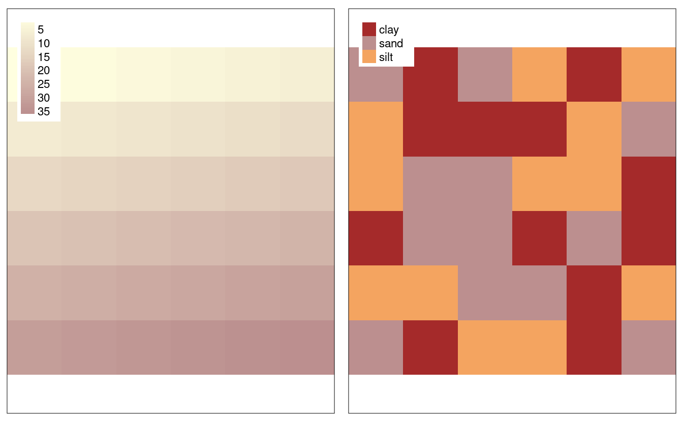
FIGURE 3.2: Raster datasets with numeric (left) and categorical values (right).
3.3.1 Raster subsetting
Raster subsetting is done with the base R operator [, which accepts a variety of inputs:
- Row-column indexing
- Cell IDs
- Coordinates (see Section 4.3.1)
- Another spatial object (see Section 4.3.1)
Here, we only show the first two options since these can be considered non-spatial operations. If we need a spatial object to subset another or the output is a spatial object, we refer to this as spatial subsetting. Therefore, the latter two options will be shown in the next chapter (see Section 4.3.1).
The first two subsetting options are demonstrated in the commands below —
both return the value of the top left pixel in the raster object elev (results not shown):
# row 1, column 1
elev[1, 1]
# cell ID 1
elev[1]
To extract all values or complete rows, you can use values() and getValues().
For multi-layered raster objects stack or brick, this will return the cell value(s) for each layer.
For example, stack(elev, grain)[1] returns a matrix with one row and two columns — one for each layer.
For multi-layer raster objects another way to subset is with raster::subset(), which extracts layers from a raster stack or brick. The [[ and $ operators can also be used:
r_stack = stack(elev, grain)
names(r_stack) = c("elev", "grain")
# three ways to extract a layer of a stack
raster::subset(r_stack, "elev")
r_stack[["elev"]]
r_stack$elev
Cell values can be modified by overwriting existing values in conjunction with a subsetting operation.
The following code chunk, for example, sets the upper left cell of elev to 0:
elev[1, 1] = 0
elev[]
#>  [1]  0  2  3  4  5  6  7  8  9 10 11 12 13 14 15 16 17 18 19 20 21 22 23 24 25
#> [26] 26 27 28 29 30 31 32 33 34 35 36
Leaving the square brackets empty is a shortcut version of values() for retrieving all values of a raster.
Multiple cells can also be modified in this way:
elev[1, 1:2] = 03.3.2 Summarizing raster objects
raster contains functions for extracting descriptive statistics for entire rasters.
Printing a raster object to the console by typing its name returns minimum and maximum values of a raster.
summary() provides common descriptive statistics (minimum, maximum, quartiles and number of NAs).
Further summary operations such as the standard deviation (see below) or custom summary statistics can be calculated with cellStats().
cellStats(elev, sd)summary() and cellStats() functions with a raster stack or brick object, they will summarize each layer separately, as can be illustrated by running: summary(brick(elev, grain)).
Raster value statistics can be visualized in a variety of ways.
Specific functions such as boxplot(), density(), hist() and pairs() work also with raster objects, as demonstrated in the histogram created with the command below (not shown):
hist(elev)In case a visualization function does not work with raster objects, one can extract the raster data to be plotted with the help of values() or getValues().
Descriptive raster statistics belong to the so-called global raster operations. These and other typical raster processing operations are part of the map algebra scheme, which are covered in the next chapter (Section 4.3.2).
Some function names clash between packages (e.g., select(), as discussed in a previous note). In addition to not loading packages by referring to functions verbosely (e.g., dplyr::select()), another way to prevent function names clashes is by unloading the offending package with detach(). The following command, for example, unloads the raster package (this can also be done in the package tab which resides by default in the right-bottom pane in RStudio): detach(“package:raster,” unload = TRUE, force = TRUE). The force argument makes sure that the package will be detached even if other packages depend on it. This, however, may lead to a restricted usability of packages depending on the detached package, and is therefore not recommended.
3.4 Exercises
For these exercises we will use the us_states and us_states_df datasets from the spData package:
library(spData)
data(us_states)
data(us_states_df)
us_states is a spatial object (of class sf), containing geometry and a few attributes (including name, region, area, and population) of states within the contiguous United States.
us_states_df is a data frame (of class data.frame) containing the name and additional variables (including median income and poverty level, for the years 2010 and 2015) of US states, including Alaska, Hawaii and Puerto Rico.
The data comes from the United States Census Bureau, and is documented in ?us_states and ?us_states_df.
- Create a new object called
us_states_namethat contains only theNAMEcolumn from theus_statesobject. What is the class of the new object and what makes it geographic? - Select columns from the
us_statesobject which contain population data. Obtain the same result using a different command (bonus: try to find three ways of obtaining the same result). Hint: try to use helper functions, such ascontainsorstarts_withfrom dplyr (see?contains). - Find all states with the following characteristics (bonus find and plot them):
- Belong to the Midwest region.
- Belong to the West region, have an area below 250,000 km2 and in 2015 a population greater than 5,000,000 residents (hint: you may need to use the function
units::set_units()oras.numeric()). - Belong to the South region, had an area larger than 150,000 km2 or a total population in 2015 larger than 7,000,000 residents.
- What was the total population in 2015 in the
us_statesdataset? What was the minimum and maximum total population in 2015? - How many states are there in each region?
- What was the minimum and maximum total population in 2015 in each region? What was the total population in 2015 in each region?
- Add variables from
us_states_dftous_states, and create a new object calledus_states_stats. What function did you use and why? Which variable is the key in both datasets? What is the class of the new object? us_states_dfhas two more rows thanus_states. How can you find them? (hint: try to use thedplyr::anti_join()function)- What was the population density in 2015 in each state? What was the population density in 2010 in each state?
- How much has population density changed between 2010 and 2015 in each state? Calculate the change in percentages and map them.
- Change the columns’ names in
us_statesto lowercase. (Hint: helper functions -tolower()andcolnames()may help.) - Using
us_statesandus_states_dfcreate a new object calledus_states_sel. The new object should have only two variables -median_income_15andgeometry. Change the name of themedian_income_15column toIncome. - Calculate the change in the number of residents living below the poverty level between 2010 and 2015 for each state. (Hint: See ?us_states_df for documentation on the poverty level columns.) Bonus: Calculate the change in the percentage of residents living below the poverty level in each state.
- What was the minimum, average and maximum state’s number of people living below the poverty line in 2015 for each region? Bonus: What is the region with the largest increase in people living below the poverty line?
- Create a raster from scratch with nine rows and columns and a resolution of 0.5 decimal degrees (WGS84). Fill it with random numbers. Extract the values of the four corner cells.
- What is the most common class of our example raster
grain(hint:modal())? - Plot the histogram and the boxplot of the
data(dem, package = "spDataLarge")raster.