Chapter 5 Using EMC for EAMs II - Race Models
In this example, we provide examples of race models – a class of EAMs where the model assumes a race between accumulators. Examples of race models include the linear ballistic accumulator (LBA; (brown2008simplest?)) and the racing diffusion model (RDM; (tillman?)). Compared to the DDM example, we use the same model checks and data set, so these examples are slightly shorter than the previous chapter. By the end of this chapter, we should have three models (DDM, LBA, RDM) which all nicely fit the data, and in the following chapter, we’ll show you how you can compare these differing accounts.
5.1 LBA
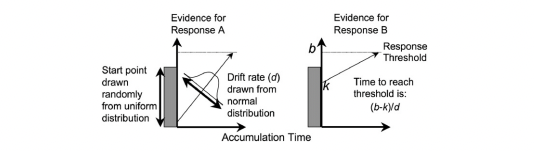
Figure 5.1: The linear ballistic accumulator model
The LBA is a “race” model of evidence accumulation, where evidence is assumed to accumulate balistically towards threshold for a number of accumulators (each representing a choice alternative). A graphical example of the model can be seen above. The LBA has similar parameters to the DDM, however, we use some slightly different names for these (consistent with the rtdists package). The parameters of the LBA are as follows;
v: Drift rate.The rate of evidence accumulation for each accumulator. For the models, we generally estimate intercept and difference terms, such that the difference is the difference in drift rate between competing accumulators. The intercept drift term is often seen as the urgency term.sv: Drift rate variance. This is the between trial variance parameter for the drift rate distribution. Typically,svis set as a constant to 1 (donkin2011response?) (however we show options below for this).B: Response threshold or response caution. The arbitrary amount of evidence needed before the corresponding response is executed. Generally,b = B + Ato ensure that threshold is greater than start point.A: Start point interval or evidence in accumulator before beginning of decision process. Start point varies from trial to trial in the interval [0, A] (uniform distribution). Average amount of evidence before evidence accumulation across trials is A/2.t0: non-decision time or response time constant (in seconds). Lower bound for the duration of all non-decisional processes (encoding and response execution).
5.1.1 LBA models in EMC (and checks)
In this section, we show a variety of models that we try for the Forstmann (2008) data, where the main factor of interest is the emphasis manipulation. We show the design functions for each of these models, some custom contrasts and then some extra checks we propose. First, let’s load in the data as before.
rm(list=ls())
setwd("EMC/")
source("emc/emc.R")
source("models/RACE/LBA/lbaB.R")

print( load("Data/PNAS.RData"))
## [1] "data" "covariates"dat <- data[,c("s","E","S","R","RT")]
names(dat)[c(1,5)] <- c("subjects","rt")
levels(dat$R) <- levels(dat$S)
# NB: This data has been truncated at 0.25s and 1.5sNow, we’re going to fit a series of models to the Forstmann (2008) data. The first model will only vary threshold with emphasis. The second varies threshold, drift and non-decision time with emphasis (saturated). The next three models include the estimation of a variability parameter sv. In the first models we set sv=1 to establish a scale.
In the three later models, we fit a series of models where sv differs between matching and mismatching accumulators, with its intercept fixed at 1 to establish scaling. Typically allowing this difference greatly improves LBA fit and results in sv_TRUE (i.e., match) > sv_FALSE. All of these designs are effect coded, so it’s worth checking out the sampled_p_vector of each model to understand which parameters are being estimated and think about how these would be mapped.
# Average rate = intercept, and rate d = difference (match-mismatch) contrast
ADmat <- matrix(c(-1/2,1/2),ncol=1,dimnames=list(NULL,"d"))

Emat <- matrix(c(0,-1,0,0,0,-1),nrow=3)
dimnames(Emat) <- list(NULL,c("a-n","a-s"))


# Only B affected by E
design_B <- make_design(
  Ffactors=list(subjects=levels(dat$subjects),S=levels(dat$S),E=levels(dat$E)),
  Rlevels=levels(dat$R),matchfun=function(d)d$S==d$lR,
  Clist=list(lM=ADmat,lR=ADmat,S=ADmat,E=Emat),
  Flist=list(v~lM,sv~1,B~E,A~1,t0~1),
  constants=c(sv=log(1)),
  model=lbaB)
# samplers <- make_samplers(dat,design_B,type="standard",rt_resolution=.02)
# save(samplers,file="sPNAS_B.RData")

# B, v and t0 affected by E
design_Bvt0 <- make_design(
  Ffactors=list(subjects=unique(dat$subjects),S=levels(dat$S),E=levels(dat$E)),
  Rlevels=levels(dat$R),matchfun=function(d)d$S==d$lR,
  Clist=list(lM=ADmat,lR=ADmat,S=ADmat,E=Emat),
  Flist=list(v~E*lM,sv~1,B~lR*E,A~1,t0~E),
  constants=c(sv=log(1)),
  model=lbaB)
# samplers <- make_samplers(dat,design_Bvt0,type="standard",rt_resolution=.02)
# save(samplers,file="sPNAS_Bvt0.RData")

# First, allowing E to affect B and t0
design_Bt0_sv <- make_design(
  Ffactors=list(subjects=unique(dat$subjects),S=levels(dat$S),E=levels(dat$E)),
  Rlevels=levels(dat$R),matchfun=function(d)d$S==d$lR,
  Clist=list(lM=ADmat,lR=ADmat,S=ADmat,E=Emat),
  Flist=list(v~lM,sv~lM,B~lR*E,A~1,t0~E),
  constants=c(sv=log(1)),
  model=lbaB)
# samplers <- make_samplers(dat,design_Bt0_sv,type="standard",rt_resolution=.02)
# save(samplers,file="sPNAS_Bt0_sv.RData")

# Now E affects B and v
design_Bv_sv <- make_design(
  Ffactors=list(subjects=unique(dat$subjects),S=levels(dat$S),E=levels(dat$E)),
  Rlevels=levels(dat$R),matchfun=function(d)d$S==d$lR,
  Clist=list(lM=ADmat,lR=ADmat,S=ADmat,E=Emat),
  Flist=list(v~E*lM,sv~lM,B~lR*E,A~1,t0~1),
  constants=c(sv=log(1)),
  model=lbaB)
# samplers <- make_samplers(dat,design_Bv_sv,type="standard",rt_resolution=.02)
# save(samplers,file="sPNAS_Bv_sv.RData")

# Now all three
design_Bvt0_sv <- make_design(
  Ffactors=list(subjects=unique(dat$subjects),S=levels(dat$S),E=levels(dat$E)),
  Rlevels=levels(dat$R),matchfun=function(d)d$S==d$lR,
  Clist=list(lM=ADmat,lR=ADmat,S=ADmat,E=Emat),
  Flist=list(v~E*lM,sv~lM,B~lR*E,A~1,t0~E),
  constants=c(sv=log(1)),
  model=lbaB)
# samplers <- make_samplers(dat,design_Bvt0_sv,type="standard",rt_resolution=.02)
# save(samplers,file="sPNAS_Bvt0_sv.RData")
We can run these five models and check the fit metrics as we did in the previous chapter. The last model fails to converge (or rather some parameter were so strongly autocorrelated it would have taken an impractically large run to produce anything useful). This might happen when doing complex modelling and can be the result of several issues, however, these issues generally relate to the amount of information available. For example, if we have a model with many parameters across varying conditions, it is likely that we have less information for each cell of the estimated design, and in these scenarios, the sampler may struggle to converge. Further, if we have a low number of subjects, this will also cause difficulty.
Here we talk about autocorrelation (using the integrated autocorrelation time stat) and effective sample sizes - these are good metrics to evaluate the quality of sampling. The basic idea behind autocorrelation is that the samples in chains are not independent, so we should estimate the effective number of independent samples. This is often because new samples are based on the previous sample in an MCMC chain. If we see high autocorrelation, this may be because we have not yet reached the posterior mode for sampling or the posterior distribution is multi-modal. We can run the sampler for a very long time, which would give us a huge number of samples, and then we could assess the effective sample size (i.e., the number of independent samples). Generally however, these problems can be solved by thinking about the model being estimated.
Looking at estimates, most issues were around the a_n contrast, which might not be surprising given this had a weak manifest effect. Here we fit this model again but dropping the a_n contrast for the emphasis effects on drift and non-decision time, instead estimating an intercept and the difference between the average of accuracy and neutral and speed, a 14 parameter model.
E_AVan_s_mat <- matrix(c(1/4,1/4,-1/2),nrow=3)
dimnames(E_AVan_s_mat) <- list(NULL,c("an-s"))

design_Bvt0_sv_NOa_n <- make_design(
  Ffactors=list(subjects=unique(dat$subjects),S=levels(dat$S),E=levels(dat$E)),
  Rlevels=levels(dat$R),matchfun=function(d)d$S==d$lR,
  Clist=list(v=list(E=E_AVan_s_mat,lM=ADmat),sv=list(lM=ADmat),
             B=list(E=Emat,lR=ADmat),t0=list(E=E_AVan_s_mat)),
  Flist=list(v~E*lM,sv~lM,B~lR*E,A~1,t0~E),
  constants=c(sv=log(1)),
  model=lbaB)
# samplers <- make_samplers(dat,design_Bvt0_sv_NOa_n,type="standard",rt_resolution=.02)
# save(samplers,file="sPNAS_Bvt0_sv_NOa_n.RData")
For the sv=1 models we used a similar script as for the DDM. For the other LBA models we use a slightly “smarter” script that only fits the next stage if the previous one worked, e.g., for the Bvsv model.
Given that we have already run these models, let’s look through some functions to check whether burn-in was completed, adaptation was completed and some other checks.
# Here we test if burn in had been done previously.
#
if (is.null(attr(samplers,"burnt")) || is.na(attr(samplers,"burnt"))) {
  sPNAS_Bv_sv <- auto_burn(samplers,cores_per_chain=4)
  save(sPNAS_Bv_sv,file="sPNAS_Bv_sv.RData")
}

# Here we check if adaptation was already done
#
if (is.null(attr(sPNAS_Bv_sv,"adapted")) && !is.na(attr(sPNAS_Bv_sv,"burnt"))) {
  sPNAS_Bv_sv <- auto_adapt(sPNAS_Bv_sv,cores_per_chain=4)
  save(sPNAS_Bv_sv,file="sPNAS_Bv_sv.RData")
}

# Here we only move on to sampling of adaptation was successful
#
if (!is.null(attr(sPNAS_Bv_sv,"adapted")) && attr(sPNAS_Bv_sv,"adapted")) {
  sPNAS_Bv_sv <- auto_sample(sPNAS_Bv_sv,iter=2000,cores_per_chain=4)
  save(sPNAS_Bv_sv,file="sPNAS_Bv_sv.RData")
}
As a side note, this code below was run later after choosing this as the best model and knowing that the first 2000 iterations of the sample run had to be discarded, giving 5000*3 = 15000 good samples to work with.
sPNAS_Bv_sv <- auto_sample(sPNAS_Bv_sv,iter=4000,cores_per_chain=10)
save(sPNAS_Bv_sv,file="sPNAS_Bv_sv.RData")
ppPNAS_Bv_sv <- post_predict(sPNAS_Bv_sv,n_cores=19,subfilter=2000)
save(ppPNAS_Bv_sv,sPNAS_Bv_sv,file="sPNAS_Bv_sv.RData")
5.1.2 Inference for the LBA
For inference, lets first load in all of the models we estimated.
#### Load model results ----
setwd("~/")
print(load("Desktop/osfstorage-archive/LBA/sPNAS_B.RData"))
## [1] "sPNAS_B"print(load("Desktop/osfstorage-archive/LBA/sPNAS_Bvt0.RData"))## [1] "sPNAS_Bvt0"print(load("Desktop/osfstorage-archive/LBA/sPNAS_Bt0_sv.RData"))## [1] "sPNAS_Bt0_sv"print(load("Desktop/osfstorage-archive/LBA/sPNAS_Bv_sv.RData"))## [1] "ppPNAS_Bv_sv" "sPNAS_Bv_sv"print(load("Desktop/osfstorage-archive/LBA/sPNAS_Bvt0_sv.RData")) # Failed model, forced to adapt and sample ## [1] "sPNAS_Bvt0_sv"print(load("Desktop/osfstorage-archive/LBA/sPNAS_Bvt0_sv_NOa_n.RData"))## [1] "sPNAS_Bvt0_sv_NOa_n"setwd("~/Documents/Research/EMC_bookdown")Note that this includes one of the failed models (Bvt0_sv). It’s worth taking a look at the chains and diagnostics for this model to help identify problems in your own modelling. Comparing these estimates to a “good” run will be immediately obvious, with stuck chains, parameters not showing stationarity, low GD statistics and low effective sample sizes.
5.1.3 Model Checks
We’re now going to again go through some basic checks to see how our models fared. We’ve left notes in the code so that you are able to check these yourself and see what we saw. For the simple B model, we can use this as a comparison for the other models.
It is important to note the difference between a good model and good estimation. For any model we estimate, we need to be able to estimate it well such that we can make clear inference on the posterior. It is this posterior that dictates whether this is an accurate model of the data, and it is on the posterior that we do model comparison. If the sampling has failed, this could indicate a poor model or just poor sampling, but regardless, it is problematic to make inference when we have not reached the posterior. On the other hand, if sampling has been completed, this does not indicate a good model, only that we have reached the posterior (which could be wrong).
Note Running the check_run function will prompt you to press ‘Enter’ to see each statistic. It will also save these plots as pdf files.
#### Check convergence ----

# Aim to get 1000 good samples as a basis for model comparison (but note this
# is not enough for inference on some parameters)
check_run(sPNAS_B)

# Slow to converge, but there by 4500
check_run(sPNAS_Bvt0,subfilter = 4500,layout=c(3,3))

# Low efficiency for t0_Ea-n, t0, and B_lRd:Ea-n
check_run(sPNAS_Bt0_sv,subfilter=2000,layout=c(3,5))

# B_lRd:Ea-n, B_Ea-n, v_Ea-n, v_Ea-n:lMd all inefficient. Some slow-wave
# oscillations, definitely need longer series if using the parameter estimates
# (even though likely stationary after 2000)
check_run(sPNAS_Bv_sv,subfilter=2000,layout=c(3,5))

# After extensive burn (although not achieving Rhat < 1.2), adaptation was quick
# but chains were very poor. Decided not to pursue further.
check_run(sPNAS_Bvt0_sv,subfilter=1000)

# Burned in quickly and converged well after 1000, B_lRd:Ea-n and especially
# t0_Ean-s quite inefficient
check_run(sPNAS_Bvt0_sv_NOa_n,subfilter=1000,layout=c(3,5))
5.1.4 Model selection
We fit 5 different LBA models, and so in a standard modelling application, we would want to know which is the best model. More importantly, we would want to objectively know which model is best using some quantifiable measures. Here, we compare information criteria (IC) for 5 different models. The ICs we compare are deviance information criterion (DIC) and Bayesian predictive information criterion (BPIC). For both of these ICs, lower IC is indicative of better model fit.
IC methods are generally a “quick and dirty” method for model comparison, where model complexity is penalized “post-hoc” and the model fit is the key metric. For these metrics, we want the model to closely match the data, as this would indicate a good fit. However, ICs can potentially miss over fitting or issues related to model complexity (i.e., sometimes a simpler model does not fit quite as well, but is more flexible to potential future data, whereas a more complex model may only fit the observed data). We’ll discuss this further in the [Model Comparison with IS2] chapter.
Let’s first compare these using the compare_IC function;
compare_IC(list(B=sPNAS_B,Bvt0=sPNAS_Bvt0,Bt0sv=sPNAS_Bt0_sv,Bvsv=sPNAS_Bv_sv,
  Bvt0sv=sPNAS_Bvt0_sv_NOa_n),subfilter=list(0,4500,2000,2001:3000,1000))
## DIC wDIC BPIC wBPIC EffectiveN meanD Dmean minD
## B -15243 0 -15100 0.000 143 -15386 -15485 -15529
## Bvt0 -15946 0 -15711 0.000 236 -16182 -16336 -16418
## Bt0sv -16870 0 -16667 0.000 203 -17073 -17206 -17276
## Bvsv -17200 1 -16986 0.999 214 -17414 -17569 -17627
## Bvt0sv -17182 0 -16973 0.001 209 -17391 -17542 -17601ICs <- compare_ICs(list(B=sPNAS_B, Bvt0=sPNAS_Bvt0, Bt0sv=sPNAS_Bt0_sv,
Bvsv=sPNAS_Bv_sv, Bvt0sv=sPNAS_Bvt0_sv_NOa_n),subfilter=list(0,4500,2000,2001:3000,1000))## wDIC_B wDIC_Bvt0 wDIC_Bt0sv wDIC_Bvsv wDIC_Bvt0sv wBPIC_B wBPIC_Bvt0 wBPIC_Bt0sv wBPIC_Bvsv wBPIC_Bvt0sv
## as1t 0 0.000 0.028 0.124 0.848 0 0.000 0.030 0.068 0.901
## bd6t 0 0.000 0.000 0.592 0.408 0 0.000 0.000 0.504 0.496
## bl1t 0 0.000 0.000 0.507 0.493 0 0.000 0.000 0.614 0.386
## hsft 0 0.000 0.000 0.548 0.452 0 0.000 0.000 0.587 0.413
## hsgt 0 0.000 0.001 0.636 0.363 0 0.000 0.002 0.673 0.324
## kd6t 0 0.000 0.254 0.454 0.292 0 0.000 0.368 0.394 0.237
## kd9t 0 0.000 0.003 0.511 0.485 0 0.000 0.008 0.366 0.626
## kh6t 0 0.000 0.150 0.496 0.354 0 0.000 0.118 0.498 0.384
## kmat 0 0.000 0.992 0.002 0.007 0 0.000 0.998 0.000 0.001
## ku4t 0 0.001 0.000 0.688 0.311 0 0.001 0.001 0.784 0.215
## na1t 0 0.000 0.044 0.595 0.360 0 0.000 0.119 0.523 0.358
## rmbt 0 0.000 0.000 0.926 0.073 0 0.000 0.001 0.740 0.259
## rt2t 0 0.000 0.000 0.918 0.082 0 0.000 0.000 0.961 0.039
## rt3t 0 0.000 0.005 0.119 0.877 0 0.000 0.001 0.070 0.929
## rt5t 0 0.001 0.228 0.319 0.452 0 0.001 0.311 0.326 0.362
## scat 0 0.000 0.330 0.255 0.416 0 0.000 0.332 0.217 0.452
## ta5t 0 0.000 0.000 0.945 0.055 0 0.000 0.000 0.959 0.041
## vf1t 0 0.000 0.000 0.867 0.133 0 0.000 0.000 0.858 0.142
## zk1t 0 0.000 0.020 0.869 0.111 0 0.000 0.003 0.790 0.207Comparing all 5 models, clearly we need sv (NB: use only 1000 from Bvsv after convergence, more added for parameter inference as this is the winning model). We noted this above, as the sv parameter often helps to capture some noise in the distributions. Let’s now try this across subjects. The latter function returns a list of matrices for each participant, so we can use that to count winners as follows.
table(unlist(lapply(ICs,function(x){row.names(x)[which.min(x$DIC)]})))##
## Bt0sv Bvsv Bvt0sv
## 1 14 4table(unlist(lapply(ICs,function(x){row.names(x)[which.min(x$BPIC)]})))##
## Bt0sv Bvsv Bvt0sv
## 1 13 5Again here we see mostly Bvsv winning, second Bvt0sv with no Ea_n, and one clear Bt0sv. We could try the simpler E contrast with the Bvsv model, but we are going to leave that as an extension exercise for you try. Now that we know the best LBA model, let’s compare this LBA model to the best fitting DDM. Let’s first load in the DDM
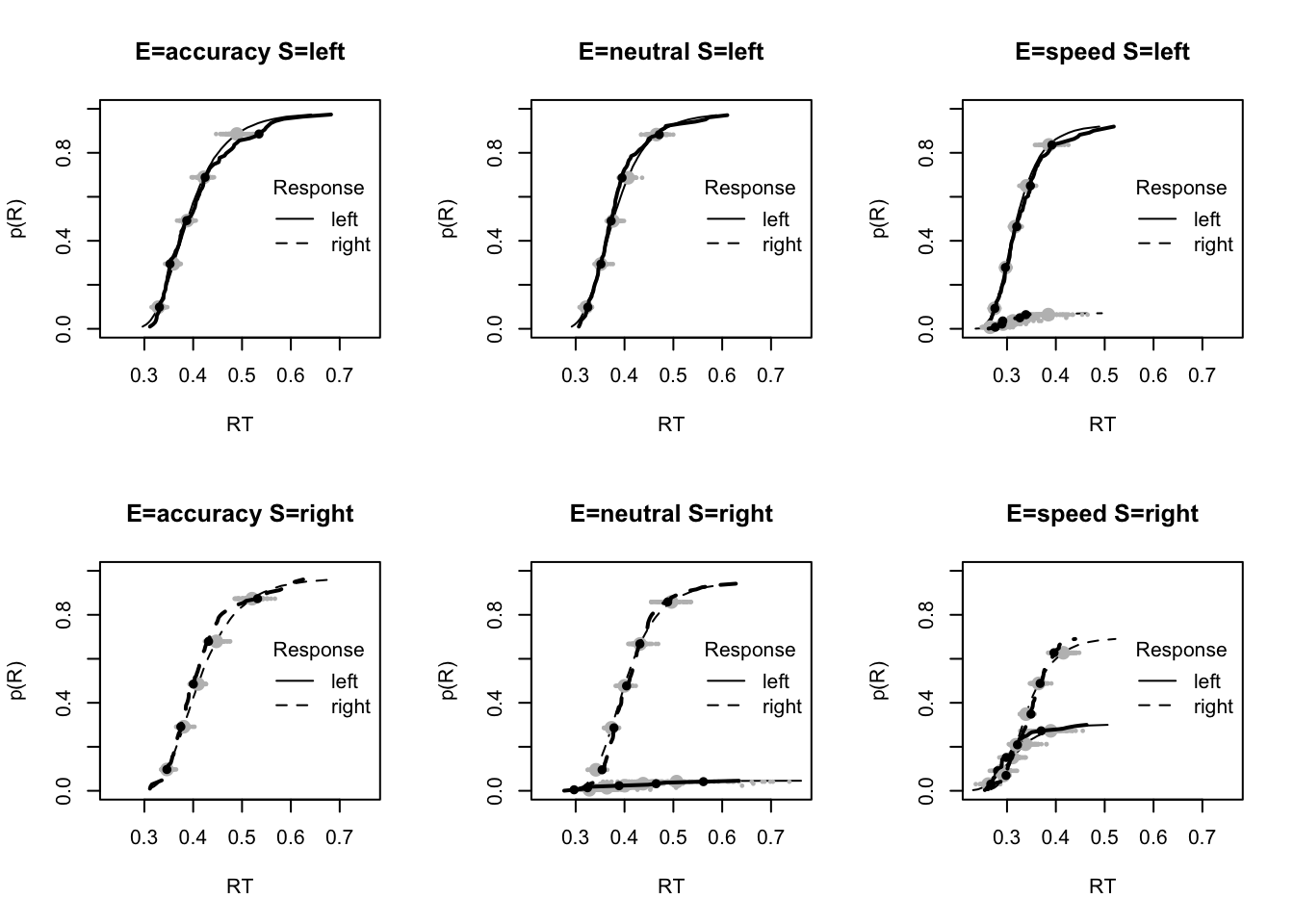
Comparing the best (by IC methods) DDM (16 parameters) to the best (15 parameter) LBA model, we see that the latter has a slight edge. This is born out in testing fit, as we see that both models fit well but the small overestimation of error RT in the speed condition evident in the DDM is no longer evident in the LBA.
setwd("EMC/")
source("models/DDM/DDM/ddmTZD.R")
load("~/Desktop/osfstorage-archive/DDM/sPNAS_avt0_full.RData")
setwd("~/Documents/Research/EMC_bookdown")
Now we can compare the ICs of the two “best” models;
# For the remaining analysis add 4000 iterations to Bvsv model
compare_IC(list(avt0=sPNAS_avt0_full,Bvsv=sPNAS_Bv_sv),subfilter=list(500,2000))
## DIC wDIC BPIC wBPIC EffectiveN meanD Dmean minD
## avt0 -17043 0 -16802 0 240 -17283 -17468 -17523
## Bvsv -17188 1 -16964 1 224 -17412 -17564 -17636Let’s now plot the fit of the winning LBA model.
####  Fit of winning (Bvsv) model ----

# post predict did not use first 2000, so inference based on 5000*3 samples
plot_fit(dat,ppPNAS_Bv_sv,layout=c(2,3),factors=c("E","S"),lpos="right",xlim=c(.25,1.5))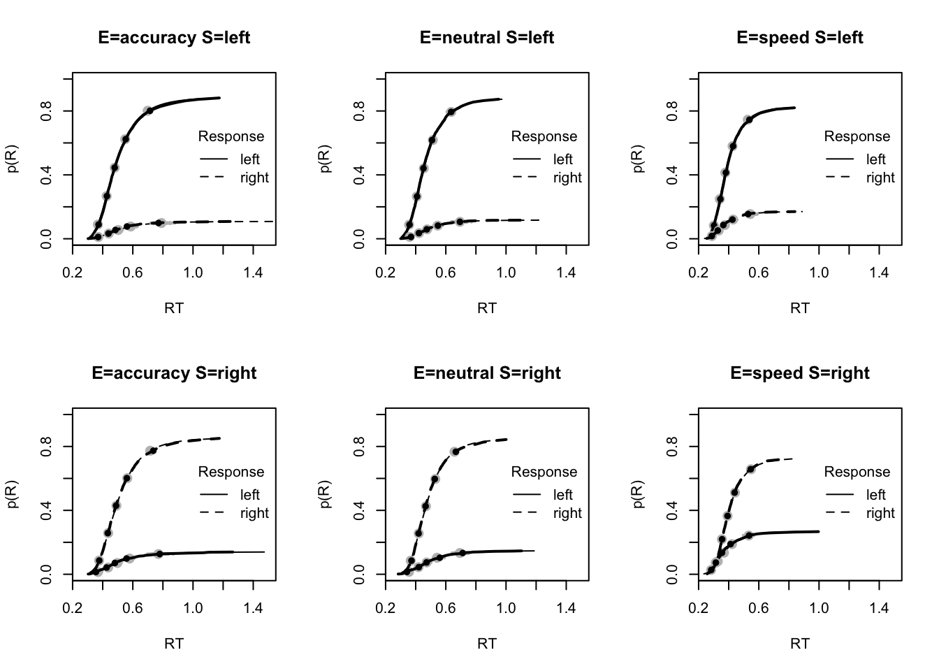
plot_fits(dat,ppPNAS_Bv_sv,layout=c(2,3),lpos="right")
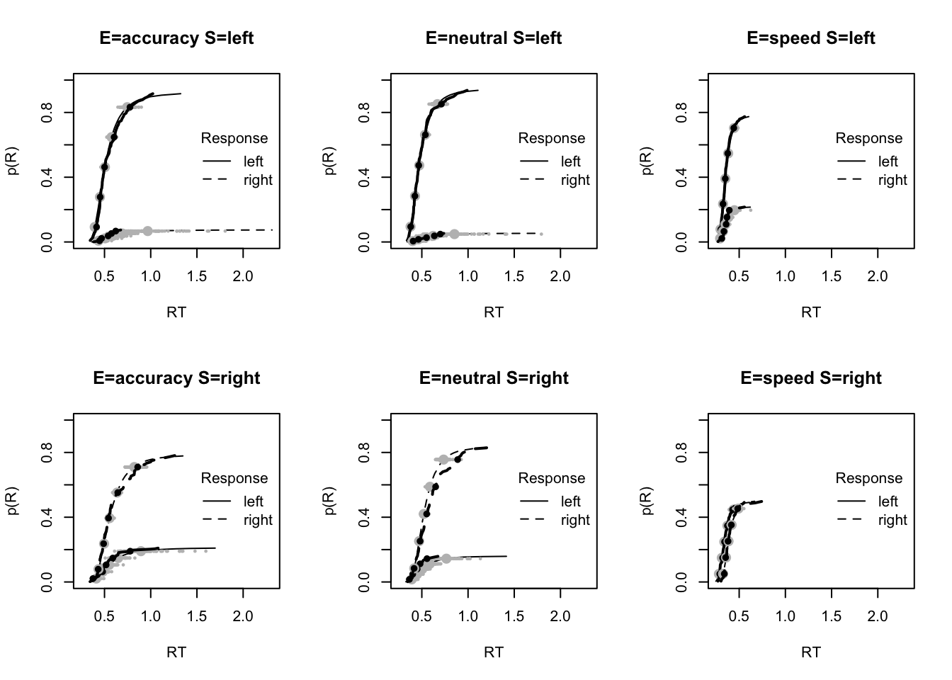
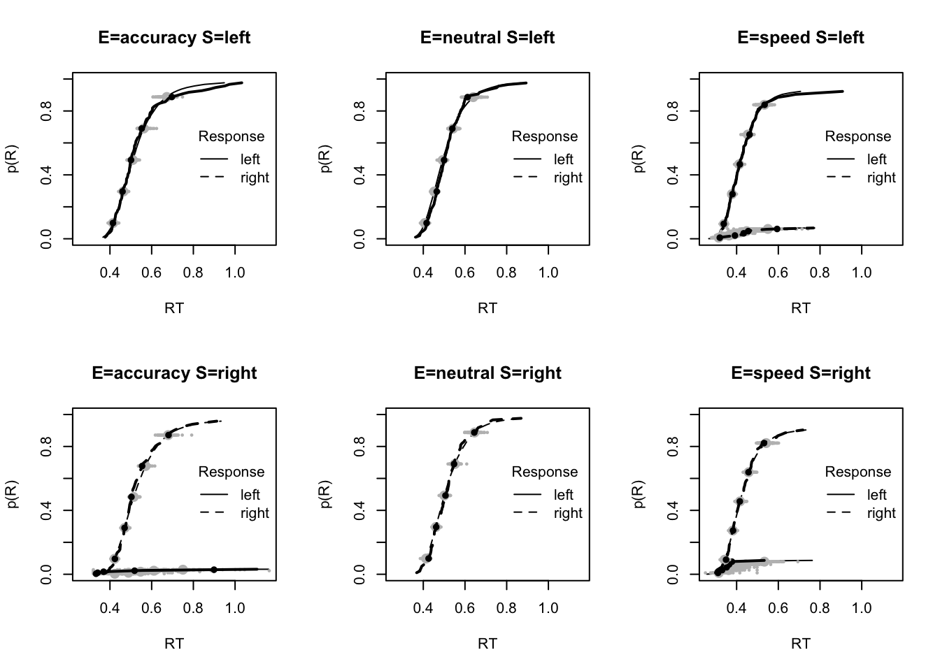
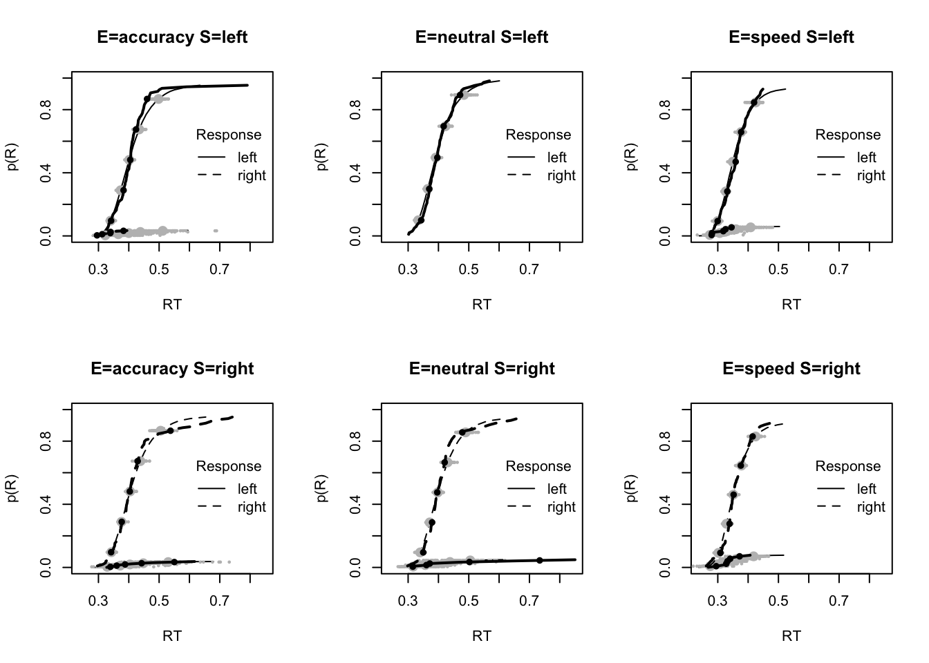
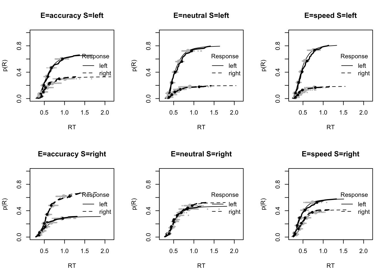
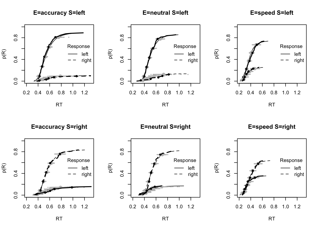
You’ll see by running the code below that there is no great evidence of misfit.
# No evidence of any misfit
pc <- function(d) 100*mean(d$S==d$R)
plot_fit(dat,ppPNAS_Bv_sv,layout=c(2,3),factors=c("E","S"),
         stat=pc,stat_name="Accuracy (%)",xlim=c(70,95))
tab <- plot_fit(dat,ppPNAS_Bv_sv,layout=c(2,3),factors=c("E","S"),
         stat=function(d){mean(d$rt)},stat_name="Mean RT (s)",xlim=c(0.375,.625))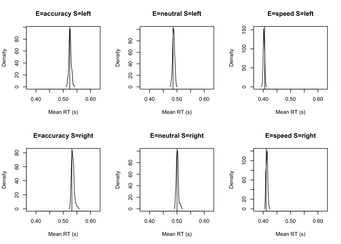
tab <- plot_fit(dat,ppPNAS_Bv_sv,layout=c(2,3),factors=c("E","S"),xlim=c(0.275,.4),
         stat=function(d){quantile(d$rt,.1)},stat_name="10th Percentile (s)")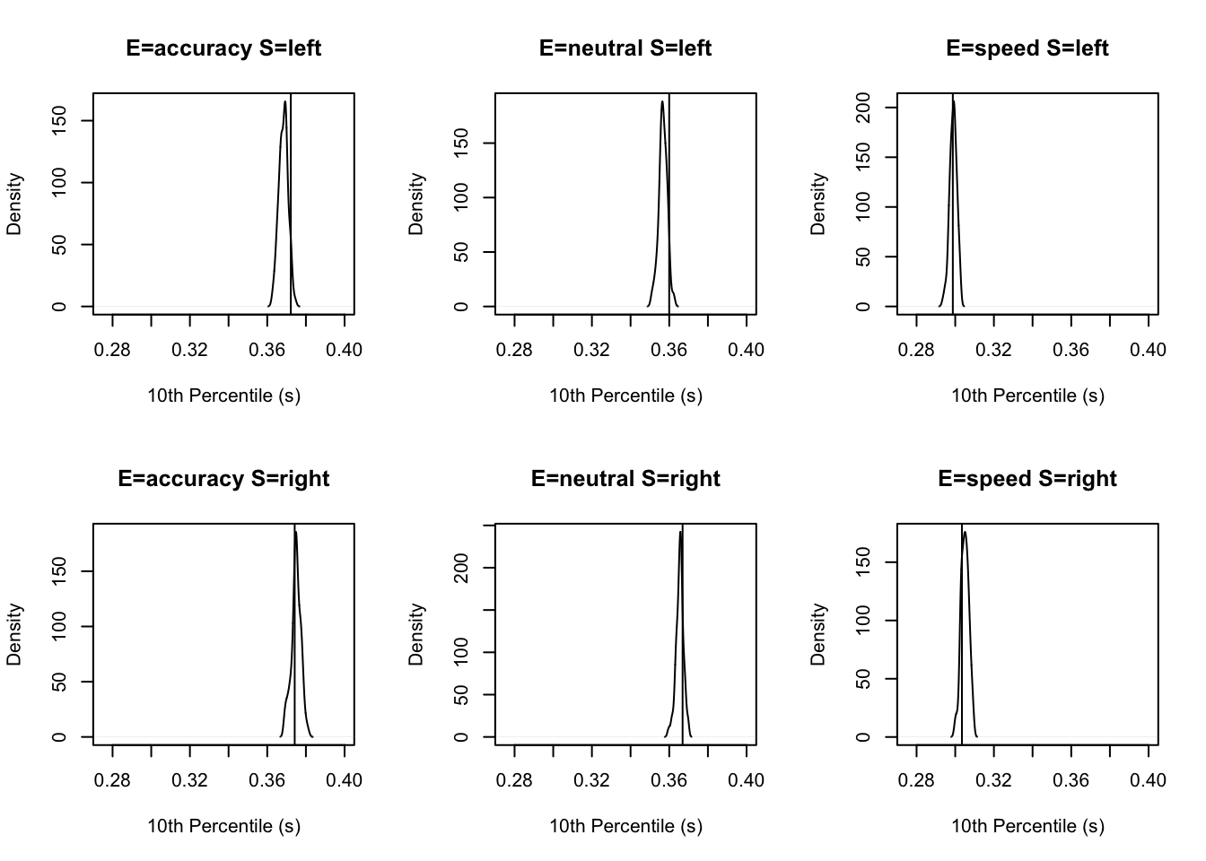
tab <- plot_fit(dat,ppPNAS_Bv_sv,layout=c(2,3),factors=c("E","S"),xlim=c(0.525,.975),
         stat=function(d){quantile(d$rt,.9)},stat_name="90th Percentile (s)")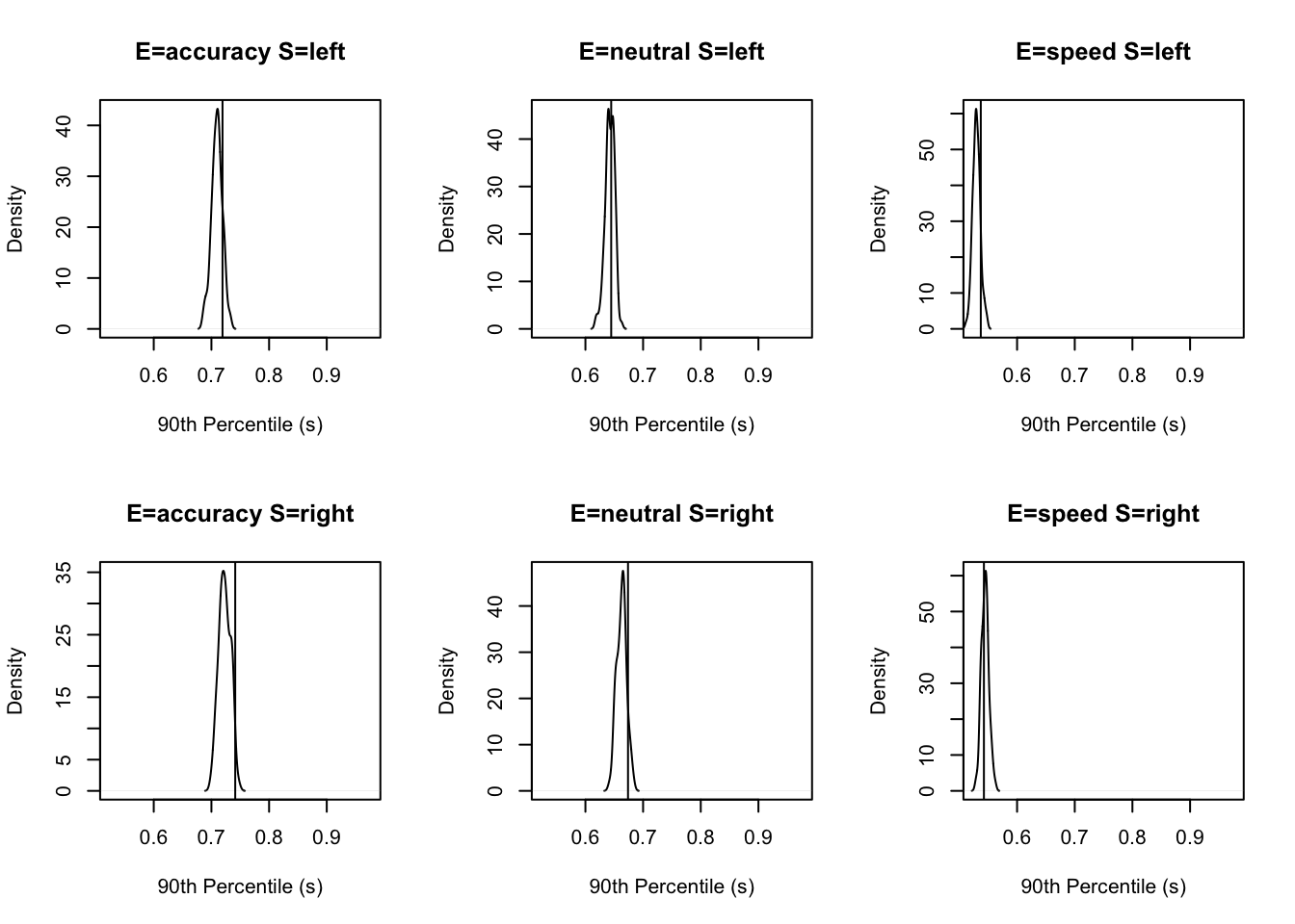
tab <- plot_fit(dat,ppPNAS_Bv_sv,layout=c(2,3),factors=c("E","S"),
         stat=function(d){sd(d$rt)},stat_name="SD (s)",xlim=c(0.1,.355))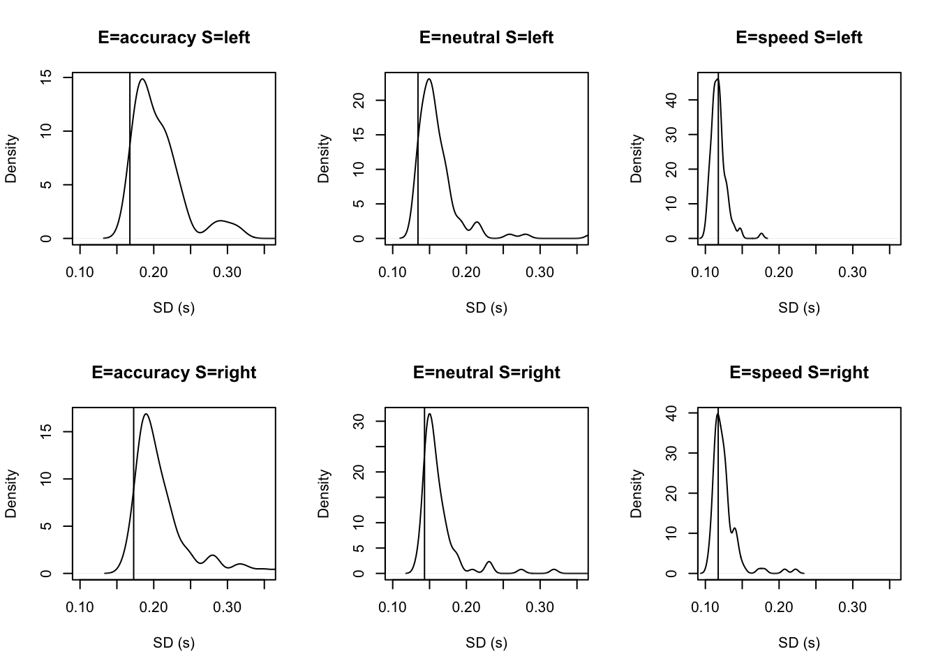
tab <- plot_fit(dat,ppPNAS_Bv_sv,layout=c(2,3),factors=c("E","S"),xlim=c(0.375,.725),
         stat=function(d){mean(d$rt[d$R!=d$S])},stat_name="Mean Error RT (s)")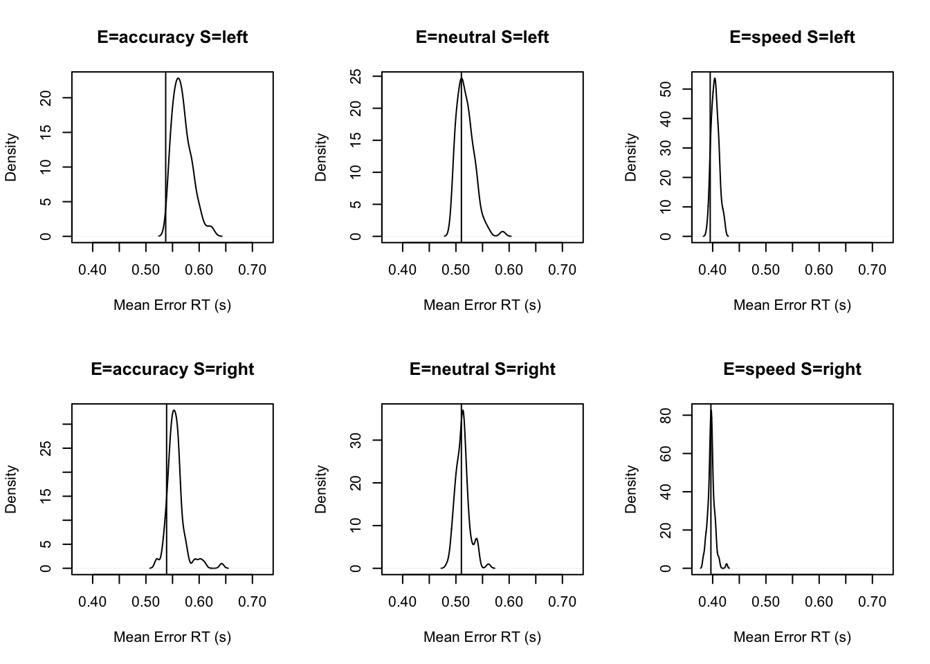
5.1.5 Posterior parameter inference
Given we are now happy with the fit of the model (relative to other models and in an absolute sense), we can begin making inference on the parameter estimates. If there is some misfit present, it is important to always contextualise inference in the level of misfit of the model to the data. Let’s start at the population level, looking at mean parameters. First we see that the priors are all well dominated except some rate parameters.
### Population mean (mu) tests

ciPNAS_Bv_sv <- plot_density(sPNAS_Bv_sv,layout=c(3,6),selection="mu",subfilter=2000)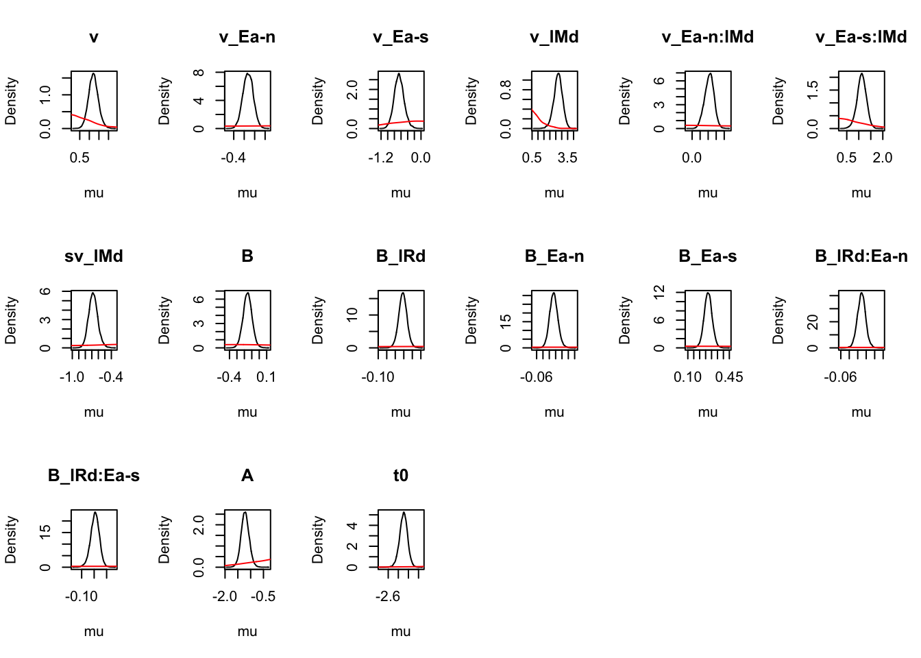
On the natural scale it is evident this is because the mismatch (FALSE) rates are least well updated, due to the fairly low error rates (errors give the most information about FALSE rates).
ciPNAS_Bv_sv_mapped <- plot_density(sPNAS_Bv_sv,layout=c(3,6),
                                        selection="mu",mapped=TRUE)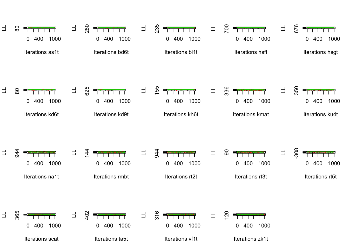
Looking at parameters both with and without mapping;
round(ciPNAS_Bv_sv,2)## v v_Ea-n v_Ea-s v_lMd v_Ea-n:lMd v_Ea-s:lMd sv_lMd B B_lRd B_Ea-n B_Ea-s B_lRd:Ea-n B_lRd:Ea-s
## 2.5% 0.73 -0.36 -0.94 1.94 0.10 0.72 -0.81 -0.28 -0.01 -0.03 0.20 -0.03 -0.08
## 50% 1.21 -0.26 -0.66 2.70 0.22 1.12 -0.68 -0.16 0.04 -0.01 0.27 -0.01 -0.05
## 97.5% 1.74 -0.17 -0.35 3.38 0.32 1.49 -0.53 -0.04 0.09 0.02 0.34 0.01 -0.01
## A t0
## 2.5% -1.52 -2.46
## 50% -1.22 -2.30
## 97.5% -0.90 -2.15round(ciPNAS_Bv_sv_mapped,2)## v_accuracy_TRUE v_accuracy_FALSE v_neutral_TRUE v_neutral_FALSE v_speed_TRUE v_speed_FALSE sv_TRUE
## 2.5% 2.25 -0.92 2.42 -0.50 2.37 0.54 0.67
## 50% 2.55 -0.14 2.71 0.24 2.65 1.08 0.71
## 97.5% 2.86 0.73 3.01 1.06 2.94 1.66 0.77
## sv_FALSE B_left_accuracy B_right_accuracy B_left_neutral B_right_neutral B_left_speed B_right_speed
## 2.5% 1.3 0.74 0.78 0.73 0.78 0.54 0.59
## 50% 1.4 0.83 0.87 0.84 0.88 0.62 0.68
## 97.5% 1.5 0.95 0.98 0.96 1.00 0.72 0.78
## A t0
## 2.5% 0.20 0.09
## 50% 0.29 0.10
## 97.5% 0.41 0.12For simpler estimates:
1) A’s is usually found with the LBA sv_true > sv_false
2) t0 is quite small (100ms)
3) In this case start point noise (.29) is small relative to B (which has intercept exp(-.16) = 0.85, so about 1/4 of b).
Let’s now look at the all important threshold effects. First we check the mapping to recall the parameterisation. Second we test right vs left response thresholds. Then we check the difference in thresholds between accuracy and neutral (B_Ea-n) and accuracy and speed (B_Ea-s).
# Recall the map used with
get_map(sPNAS_Bv_sv)$B
## lR E B B_lRd B_Ea-n B_Ea-s B_lRd:Ea-n B_lRd:Ea-s
## 1 left accuracy 1 -0.5 0 0 0.0 0.0
## 7 right accuracy 1 0.5 0 0 0.0 0.0
## 2 left neutral 1 -0.5 -1 0 0.5 0.0
## 8 right neutral 1 0.5 -1 0 -0.5 0.0
## 3 left speed 1 -0.5 0 -1 0.0 0.5
## 9 right speed 1 0.5 0 -1 0.0 -0.5# B_lRd tests threshold right - threshold left, although not quite credible
# it indicates slightly higher right thresholds (i.e., a bias to respond left)
p_test(x=sPNAS_Bv_sv,x_name="B_lRd",subfilter=2000)## B_lRd mu
## 2.5% -0.01 NA
## 50% 0.04 0
## 97.5% 0.09 NA
## attr(,"less")
## [1] 0.037# B_Ea-n and B_Ea-s measure differences in response caution (i.e., thresholds
# averaged over left and right accumulators), accuracy-neutral and accuracy-speed
# respectively. Caution for accuracy is clearly higher than speed, but not
# credibly greater than neutral.
p_test(x=sPNAS_Bv_sv,x_name="B_Ea-n",subfilter=2000)## B_Ea-n mu
## 2.5% -0.03 NA
## 50% -0.01 0
## 97.5% 0.02 NA
## attr(,"less")
## [1] 0.69p_test(x=sPNAS_Bv_sv,x_name="B_Ea-s",subfilter=2000)## B_Ea-s mu
## 2.5% 0.20 NA
## 50% 0.27 0
## 97.5% 0.34 NA
## attr(,"less")
## [1] 0There are several other tests for thresholds that we could report on. Try these out for yourself by using the code below;
# Here we construct a test showing the processing speed
# advantage is greater for speed than neutral
p_test(x=sPNAS_Bv_sv,mapped=TRUE,x_name="average B: neutral-speed",
  x_fun=function(x){mean(x[c("B_left_neutral","B_right_neutral")]) -
                    mean(x[c("B_left_speed","B_right_speed")])})

# No evidence of a difference between accuracy and neutral thresholds
p_test(x=sPNAS_Bv_sv,x_name="B_Ea-n",subfilter=2000)

# But thresholds clearly higher for speed (by about 0.2 on the natural scale)
p_test(x=sPNAS_Bv_sv,x_name="B_Ea-s",subfilter=2000)

# The remaining terms test interactions with bias (i.e., lR), with evidence of
# a small but just credibly stronger bias to respond left (i.e., a lower threshold
# for the left accumulator) for speed than accuracy.
p_test(x=sPNAS_Bv_sv,x_name="B_lRd:Ea-s",subfilter=1500,digits=2)
Next, lets look at drift rate effects. For these, we’ll again look at the mapping first, and then look at the difference parameters between accuracy and neutral or speed conditions.
# Again recall the map used with
get_map(sPNAS_Bv_sv)$v
## E lM v v_Ea-n v_Ea-s v_lMd v_Ea-n:lMd v_Ea-s:lMd
## 1 accuracy TRUE 1 0 0 0.5 0.0 0.0
## 7 accuracy FALSE 1 0 0 -0.5 0.0 0.0
## 2 neutral TRUE 1 -1 0 0.5 -0.5 0.0
## 8 neutral FALSE 1 -1 0 -0.5 0.5 0.0
## 3 speed TRUE 1 0 -1 0.5 0.0 -0.5
## 9 speed FALSE 1 0 -1 -0.5 0.0 0.5# v_Ea-n v_Ea-s indicate that processing rate (the average of matching and
# mismatching rates) is least in accuracy, slightly greater in neutral and
# the highest in speed.
p_test(x=sPNAS_Bv_sv,x_name="v_Ea-n",subfilter=2000)## v_Ea-n mu
## 2.5% -0.36 NA
## 50% -0.26 0
## 97.5% -0.17 NA
## attr(,"less")
## [1] 1p_test(x=sPNAS_Bv_sv,x_name="v_Ea-s",subfilter=2000)## v_Ea-s mu
## 2.5% -0.94 NA
## 50% -0.66 0
## 97.5% -0.35 NA
## attr(,"less")
## [1] 1Again we show additional tests you could do below;
# Here we show that processing is faster in the speed condition.
p_test(x=sPNAS_Bv_sv,mapped=TRUE,x_name="average v: speed-neutral",
  x_fun=function(x){mean(x[c("v_speed_TRUE","v_speed_FALSE")]) -
                    mean(x[c("v_neutral_TRUE","v_neutral_FALSE")])})

# v_lMd tests the quality of selective attention, rate match - rate mismatch
p_test(x=sPNAS_Bv_sv,x_name="v_lMd",subfilter=2000)

# v_Ea-n tests if quality neutral - quality accuracy (i.e,
# (2.55 - -0.14) - (2.71  - 0.24) = 0.22)
p_test(x=sPNAS_Bv_sv,x_name="v_Ea-n:lMd",subfilter=2000)

# The difference is ~5 times larger for accuracy - speed
p_test(x=sPNAS_Bv_sv,x_name="v_Ea-s:lMd",subfilter=2000)

# The neutral - speed difference is also highly credible, and
# can be tested in the mapped form
p_test(x=sPNAS_Bv_sv,mapped=TRUE,x_name="quality: accuracy-neutral",
  x_fun=function(x){diff(x[c("v_neutral_FALSE","v_neutral_TRUE")]) -
                    diff(x[c("v_speed_FALSE","v_speed_TRUE")])})
# Or from the sampled parameters (i.e., 1.12 - .22)
p_test(x=sPNAS_Bv_sv,x_name="v_Ea-s:lMd",y=sPNAS_Bv_sv,y_name="v_Ea-n:lMd",
       subfilter=2000,digits=3)
5.2 RDM
The Racing Diffusion Model (RDM) is a model which utilises both the race structure and diffusion model framework. Here, we use a diffusion process towards a single threshold for each accumulator of the model. A grpahical example can be seen below.
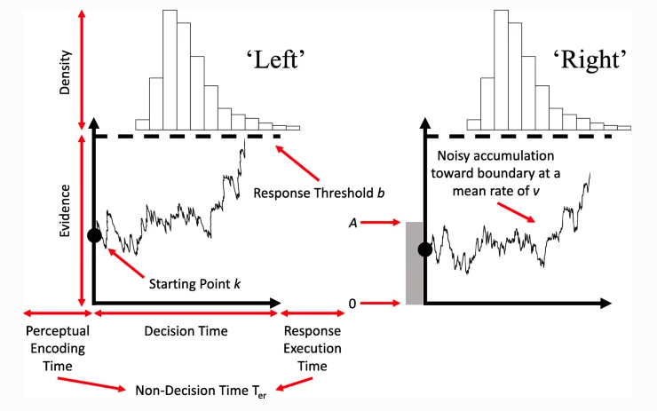
Figure 5.2: The racing diffusion model
5.2.1 RDM in EMC
To use the RDM, we show the a similar structure as we did for the LBA and LNR. First, let’s prepare our environment.
rm(list=ls())
setwd("EMC/")
source("emc/emc.R")
source("models/RACE/RDM/rdmB.R")

print( load("Data/PNAS.RData"))
dat <- data[,c("s","E","S","R","RT")]
names(dat)[c(1,5)] <- c("subjects","rt")
levels(dat$R) <- levels(dat$S)
5.2.2 RDM Model Design
Now we can look at the design for our model. The parameters we specify for the RDM are very similar to the LBA, with v the mean rate of evidence accumulation, B the threshold, A the start point and t0 the non-decision time. We can also include additional variability parameters as is shown below.
In this code, we again show several different types of model designs that vary different parameters. These include a thresholds only model; threshold, drift and t0 model; threshold and t0 model; and a threshold and drift model.
# Average and difference matrix
ADmat <- matrix(c(-1/2,1/2),ncol=1,dimnames=list(NULL,"d"))

Emat <- matrix(c(0,-1,0,0,0,-1),nrow=3)
dimnames(Emat) <- list(NULL,c("a-n","a-s"))

design_B <- make_design(
  Ffactors=list(subjects=levels(dat$subjects),S=levels(dat$S),E=levels(dat$E)),
  Rlevels=levels(dat$R),matchfun=function(d)d$S==d$lR,
  Clist=list(lM=ADmat,lR=ADmat,S=ADmat,E=Emat),
  Flist=list(v~lM,B~lR*E,A~1,t0~1),
  model=rdmB)


design_Bvt0<- make_design(
  Ffactors=list(subjects=levels(dat$subjects),S=levels(dat$S),E=levels(dat$E)),
  Rlevels=levels(dat$R),matchfun=function(d)d$S==d$lR,
  Clist=list(lM=ADmat,lR=ADmat,S=ADmat,E=Emat),
  Flist=list(v~lM*E,B~lR*E,A~1,t0~E),
  model=rdmB)

design_Bt0<- make_design(
  Ffactors=list(subjects=levels(dat$subjects),S=levels(dat$S),E=levels(dat$E)),
  Rlevels=levels(dat$R),matchfun=function(d)d$S==d$lR,
  Clist=list(lM=ADmat,lR=ADmat,S=ADmat,E=Emat),
  Flist=list(v~lM,B~lR*E,A~1,t0~E),
  model=rdmB)


design_Bv<- make_design(
  Ffactors=list(subjects=levels(dat$subjects),S=levels(dat$S),E=levels(dat$E)),
  Rlevels=levels(dat$R),matchfun=function(d)d$S==d$lR,
  Clist=list(lM=ADmat,lR=ADmat,S=ADmat,E=Emat),
  Flist=list(v~lM*E,B~lR*E,A~1,t0~1),
  model=rdmB)

# rdm_B <- make_samplers(dat,design_B,type="standard",rt_resolution=.02)
# rdm_Bvt0<- make_samplers(dat,design_Bvt0,type="standard",rt_resolution=.02)
# rdm_Bt0 <- make_samplers(dat,design_Bt0,type="standard",rt_resolution=.02)
# rdm_Bv <- make_samplers(dat,design_Bv,type="standard",rt_resolution=.02)
#
All of these models are run in a single file, run_rdm.R using the run_emc function. This function is given the name of the file containing the samplers object and any arguments to its constituent functions (auto_burn, auto_adapt and auto_sample). For example the first model was fit with 8 cores per chain and so 24 cores in total given the default of 3 chains.
run_emc(“rdmPNAS_B.RData”,cores_per_chain=8)
If any stage failsrun_check stops, saving the progress so far. The only argument unique to this function is nsample, which determines the number of iterations performed if the sample stage is reached (by default 1000).
After the convergence checking reported below extra samples were obtained for some models that converged slowly, so all had 1000 converged samples. This was done by adding another run_emc call with nsamples set appropriately (run_emc recognizes that burn and adapt stages are complete and so just adds on the extra samples at the end).
Finally for the selected model extra samples were added to obtain 5000 iterations, so posterior inference was reliable, and posterior predictives were obtained. (NB: if the file is run several times some lines must be commented out or unwanted sample stage iteration will be added)
#### Check convergence ----
print(load("models/RACE/RDM/examples/samples/rdmPNAS_B.RData"))
print(load("models/RACE/RDM/examples/samples/rdmPNAS_Bt0.RData"))
print(load("models/RACE/RDM/examples/samples/rdmPNAS_Bv.RData"))
print(load("models/RACE/RDM/examples/samples/rdmPNAS_Bvt0.RData"))
check_run(rdm_B)
check_run(rdm_Bt0,subfilter=500)
check_run(rdm_Bv,subfilter=1500)
check_run(rdm_Bvt0,subfilter=1500)
#### Model selection ----
# Bvt0 wins with Bt0 second
compare_IC(list(B=rdm_B,Bt0=rdm_Bt0,Bv=rdm_Bv,Bvt0=rdm_Bvt0),
subfilter=list(0,500,1500,1500))
# But at the subject level Bv is second
ICs <- compare_ICs(list(B=rdm_B,Bt0=rdm_Bt0,Bv=rdm_Bv,Bvt0=rdm_Bvt0),
subfilter=list(0,500,1500,1500:2500))
table(unlist(lapply(ICs,function(x){row.names(x)[which.min(x$DIC)]})))
table(unlist(lapply(ICs,function(x){row.names(x)[which.min(x$BPIC)]})))
# Comparing with the best DDM (16 parameter) model to the best (15 parameter)
# LBA model and best (16 parameter) RDM the latter comes third.
source("models/DDM/DDM/ddmTZD.R")
print(load("models/DDM/DDM/examples/samples/sPNAS_avt0_full.RData"))
source("models/RACE/LBA/lbaB.R")
print(load("models/RACE/LBA/examples/samples/sPNAS_Bv_sv.RData"))
compare_IC(list(DDM_avt0=sPNAS_avt0_full,LBA_Bvsv=sPNAS_Bv_sv,RDM_Bvt0=rdm_Bvt0),
subfilter=list(500,2000,1500))
# For the remaining analysis add 4000 iterations to Bvt0 model
#### Fit of winning (Bvsv) model ----
# post predict did not use first 1500, so inference based on 5000*3 samples
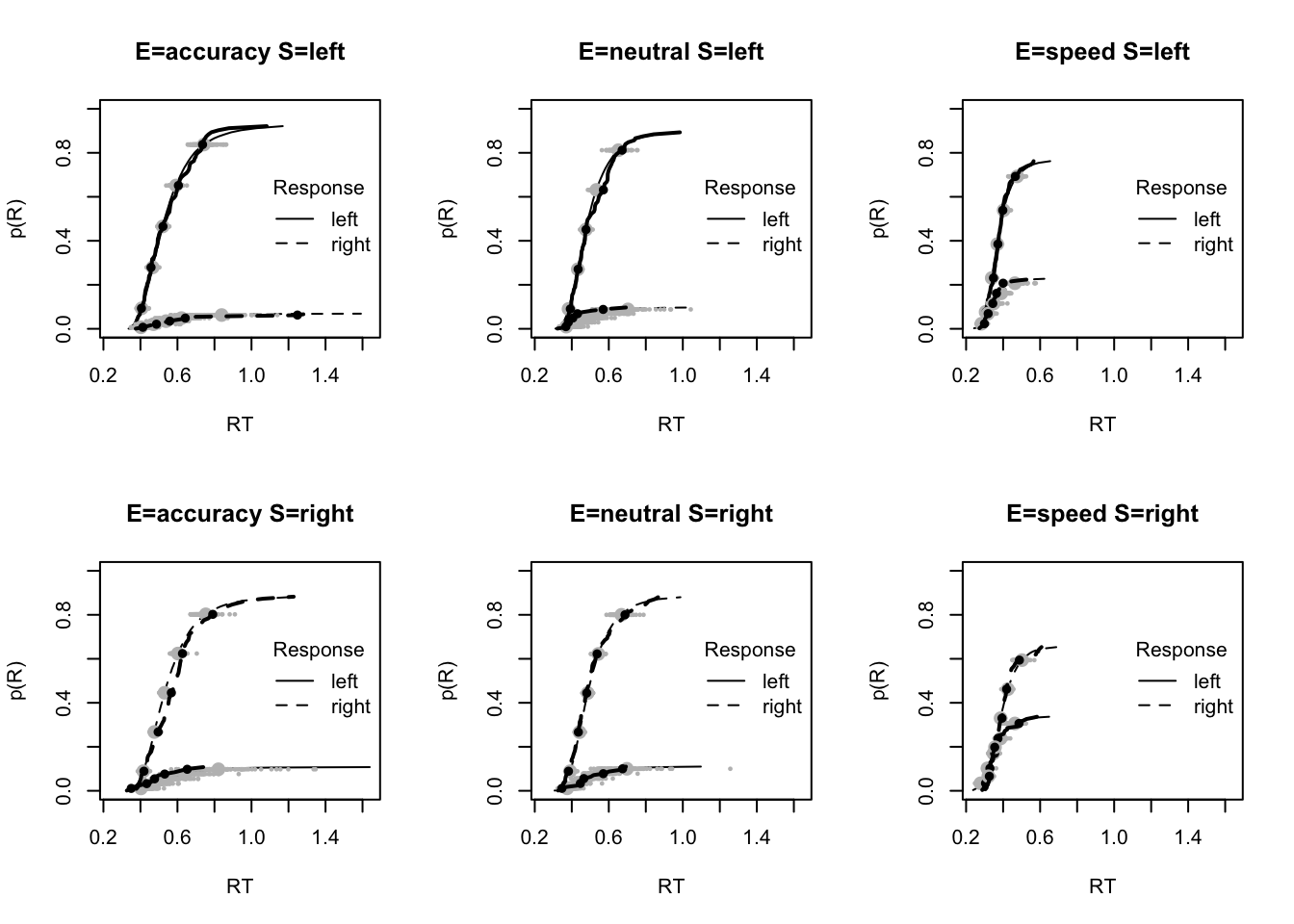
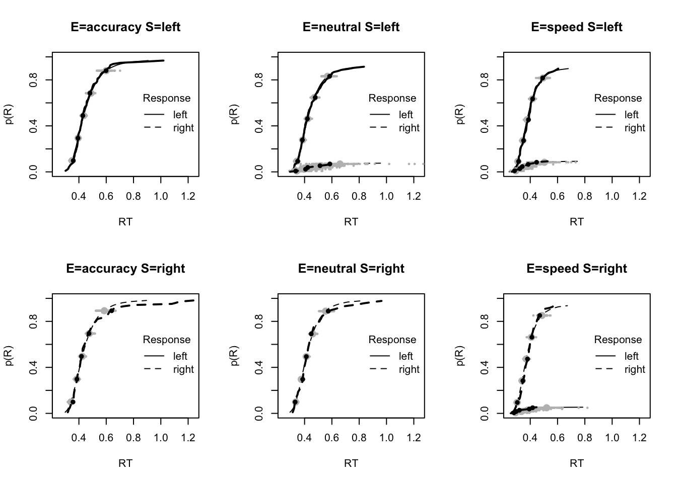
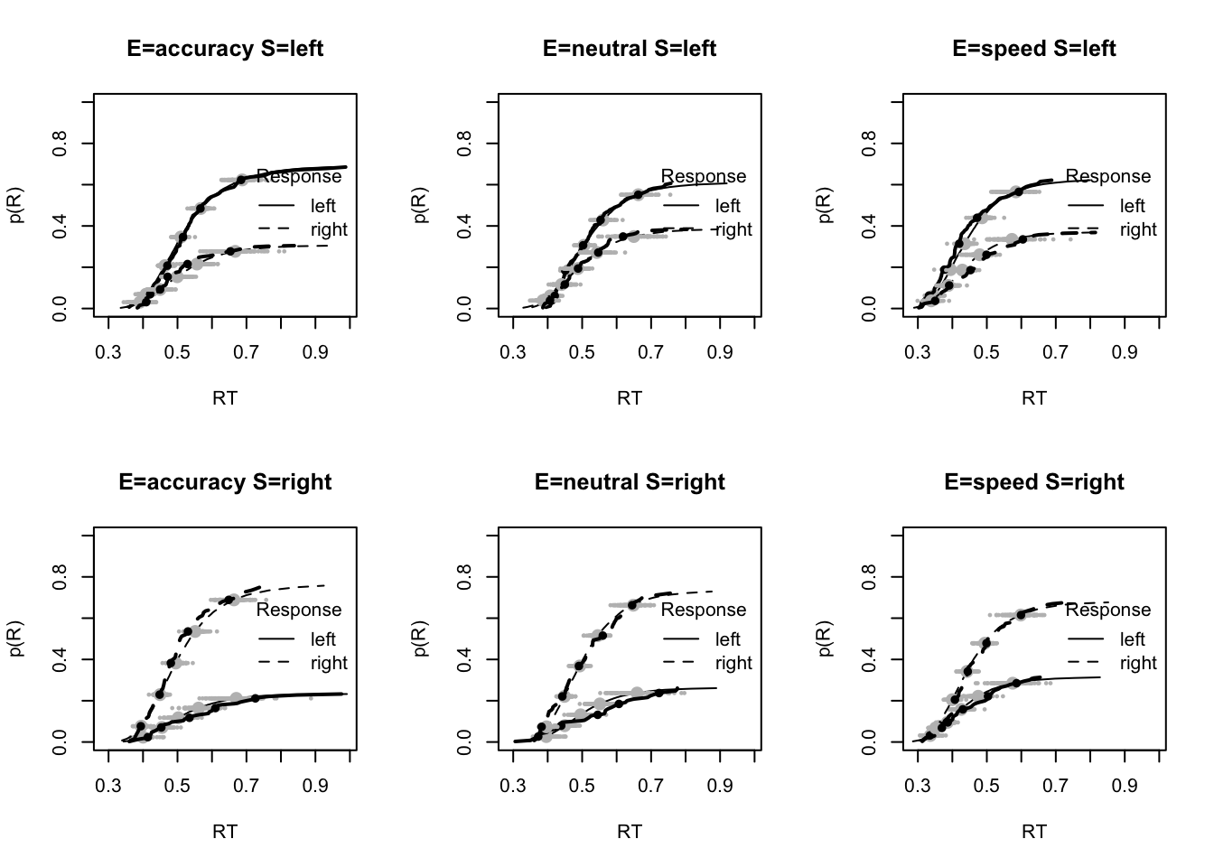
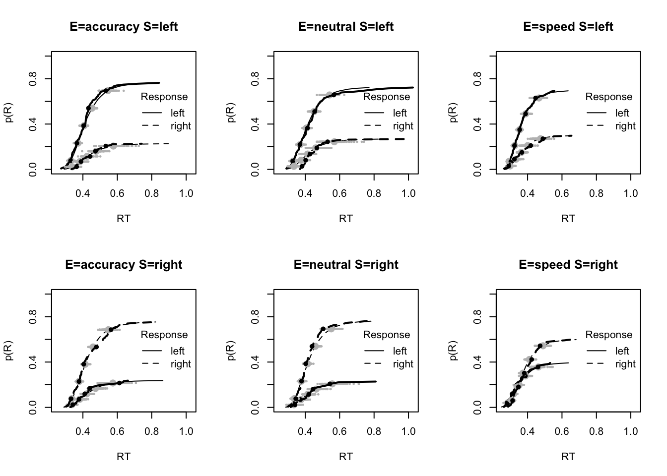
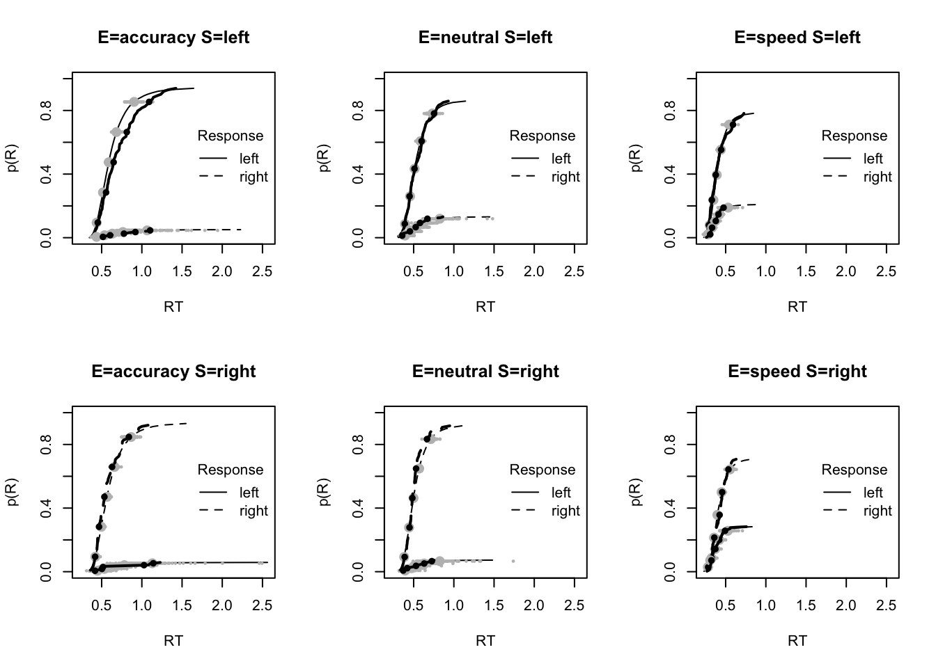
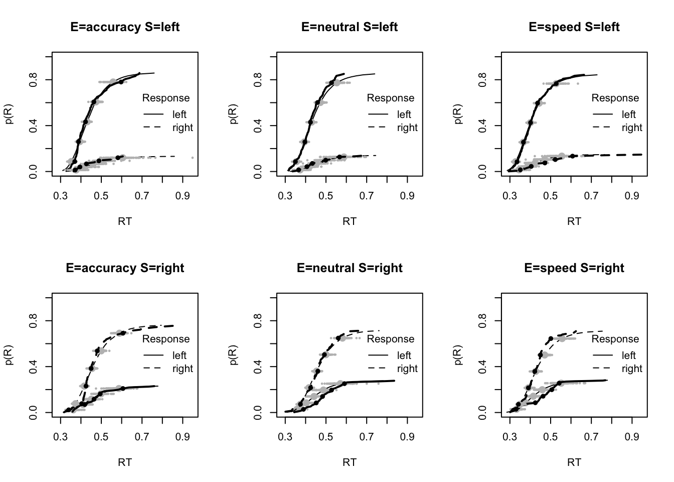
plot_fit(dat,pprdm_Bvt0,layout=c(2,3),factors=c("E","S"),lpos="right",xlim=c(.25,1.5))
plot_fits(dat,pprdm_Bvt0,layout=c(2,3),lpos="right")
# Good fit, slight under-estimation of 10th percentile and over-estimation of
# error RT in speed
pc <- function(d) 100*mean(d$S==d$R)
plot_fit(dat,pprdm_Bvt0,layout=c(2,3),factors=c("E","S"),
stat=pc,stat_name="Accuracy (%)",xlim=c(70,95))
tab <- plot_fit(dat,pprdm_Bvt0,layout=c(2,3),factors=c("E","S"),
stat=function(d){mean(d$rt)},stat_name="Mean RT (s)",xlim=c(0.375,.625))
tab <- plot_fit(dat,pprdm_Bvt0,layout=c(2,3),factors=c("E","S"),xlim=c(0.275,.4),
stat=function(d){quantile(d$rt,.1)},stat_name="10th Percentile (s)")
tab <- plot_fit(dat,pprdm_Bvt0,layout=c(2,3),factors=c("E","S"),xlim=c(0.525,.975),
stat=function(d){quantile(d$rt,.9)},stat_name="90th Percentile (s)")
tab <- plot_fit(dat,pprdm_Bvt0,layout=c(2,3),factors=c("E","S"),
stat=function(d){sd(d$rt)},stat_name="SD (s)",xlim=c(0.1,.355))
tab <- plot_fit(dat,pprdm_Bvt0,layout=c(2,3),factors=c("E","S"),xlim=c(0.375,.725),
stat=function(d){mean(d$rt[d$R!=d$S])},stat_name="Mean Error RT (s)")
#### Posterior parameter inference ----
### Population mean (mu) tests
# Priors all well dominated except some rate parameters
cirdm_Bvt0 <- plot_density(rdm_Bvt0,layout=c(3,6),selection="mu",subfilter=1500)
# On the natural scale it is evident this is because the mismatch (FALSE) rates
# are least well updated, due to the fairly low error rates (errors give the
# most information about FALSE rates).
cirdm_Bvt0_mapped <- plot_density(rdm_Bvt0,layout=c(3,6),
selection="mu",mapped=TRUE)
# Looking at parameters both with and without mapping
round(cirdm_Bvt0,2)
round(cirdm_Bvt0_mapped,2)
# For simpler estimates:
# 1) t0 is longer than the LBA
# 2) Start point noise slightly larger relative to B than for the LBA.
### B effects
# Recall the map used with
get_map(rdm_Bvt0)$B
# B_lRd tests threshold right - threshold left, as for the LBA, although not
# quite credible it indicates slightly higher right thresholds (i.e., a bias to
# respond left)
p_test(x=rdm_Bvt0,x_name="B_lRd",subfilter=1500,digits=3)
# B_Ea-n and B_Ea-s measure differences in response caution (i.e., thresholds
# averaged over left and right accumulators), accuracy-neutral and accuracy-speed
# respectively. Caution for accuracy is clearly higher than speed, but not
# credibly greater than neutral.
p_test(x=rdm_Bvt0,x_name="B_Ea-n",subfilter=1500)
p_test(x=rdm_Bvt0,x_name="B_Ea-s",subfilter=1500)
# Here we construct a test on the natural scale showing caution is greater for
# neutral than speed
p_test(x=rdm_Bvt0,mapped=TRUE,x_name="average B: neutral-speed",
x_fun=function(x){mean(x[c("B_left_neutral","B_right_neutral")]) -
mean(x[c("B_left_speed","B_right_speed")])})
# The remaining terms test interactions with bias (i.e., lR), with evidence of
# a small but credibly stronger bias to respond left (i.e., a lower threshold
# for the left accumulator) for speed than accuracy.
p_test(x=rdm_Bvt0,x_name="B_lRd:Ea-s",subfilter=1500,digits=2)
### v effects
# Again recall the map used with
get_map(rdm_Bvt0)$v
# v_Ea-n v_Ea-s indicate that processing rate (the average of matching and
# mismatching rates) is less in the accuracy condition than in neutral or speed.
p_test(x=rdm_Bvt0,x_name="v_Ea-n",subfilter=1500)
p_test(x=rdm_Bvt0,x_name="v_Ea-s",subfilter=1500)
# However, neutral and speed do not credibly differ
p_test(x=rdm_Bvt0,mapped=TRUE,x_name="average v: speed-neutral",
x_fun=function(x){mean(x[c("v_TRUE_speed","v_FALSE_speed")]) -
mean(x[c("v_TRUE_neutral","v_FALSE_neutral")])})
# v_lMd tests the quality of selective attention, rate match - rate mismatch
p_test(x=rdm_Bvt0,x_name="v_lMd",subfilter=1500)
# v_Ea-n indicates quality does not differ credibly between accuracy and neutral.
p_test(x=rdm_Bvt0,x_name="v_lMd:Ea-n",subfilter=1500)
# In contrast there is a strong difference for accuracy - speed
p_test(x=rdm_Bvt0,x_name="v_lMd:Ea-s",subfilter=1500)
# The neutral - speed difference is also highly credible, here is is tested
# in the mapped form
p_test(x=rdm_Bvt0,mapped=TRUE,x_name="quality: accuracy-neutral",
x_fun=function(x){diff(x[c("v_FALSE_neutral","v_TRUE_neutral")]) -
diff(x[c("v_FALSE_speed","v_TRUE_speed")])})5.3 LNR
The Lognormal distribution: a distribution whose logarithm is normal.
The log-normal distribution has long history of being used to model RT distribution with the near universal positively skewed shape evident for RT. It is another type of central limit for the product of random variables, xi. The log-normal distribution is similar to a response time distribution, but the log-normal distribution starts at 0, whereas (as we discussed above), response time should begin a bit later than that (maybe around .2 seconds). To overcome this, we can add a shift the the log-normal. For this example we will use the shifted log-normal to model RT distribution:
\(RT ~ shift + Lognormal(meanlog,sdlog)\)
$meanlog/sdlog = mean and sd $ on the log scale
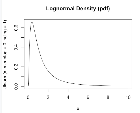
Figure 5.3: The diffusion decision model
This paper (Heathcote and Love 2012) discusses this history and how the log-normal distribution can arise from different psychological processes such as a “cascade” process where the random variable are the rates of each stage in the cascade. The paper also develops a model of choice, which we will briefly return to in subsequent chapters. The log-normal race model is the most tractable of EMC’s race models. For now, we will use the shifted log-normal to model RT distribution. For more on the log-normal race model that addresses choice processing see (Rouder et al. 2015).
5.3.1 Theory and Model
First, let’s graphically look at the log-normal distribution;
Again, this looks similar to the response time distributions we saw above. When thinking about how the “model” works, we can take the log of the distribution, which stretches out our distribution to give us something that resembles a normal distribution (which is easy to estimate);
# If you know the shift then it is easy to get estimates

# Make lots of data
pars <- c(meanlog = runif(1,-1,0), sdlog = runif(1,.5,1.5),shift=runif(1,.1,.5))
n=1e4
sdata <- pars[3]+rlnorm(n,meanlog=pars[1],sdlog=pars[2])
logsdata <- log(sdata - pars[3])
c(mean=mean(logsdata),sd=sd(logsdata))
# Even if you dont know the shift you know it will be somewhere reasonably close
# to the minimum RT
min(sdata)# Lets say we guess (conservatively) shift = 0.2
logsdata <- log(sdata - 0.2)
c(mean=mean(logsdata),sd=sd(logsdata))# We can see how this shifts things closer to normal (in these
# plots normal = straight line)
par(mfrow=c(1,3))
qqnorm(quantile(log(sdata),probs=c(1:1000)/1000))
qqnorm(quantile(log(sdata-0.2),probs=c(1:1000)/1000))
qqnorm(quantile(log(sdata-pars[3]),probs=c(1:1000)/1000))# But how can we get the shift? We could simply get the log-likelihood by
# calculating meanlog and sdlog via the moments estimators for each candidate
# shift value
estimate_slnormal <- function(data,p_range=c(0,1),npts=1000,doPlot=TRUE)
{
slnormal_loglikelihood <- function(shift,data) {
d <- data-shift
ld <- log(d)
sum(log(dlnorm(d, mean(ld),sd(ld))))
}
x <- seq(p_range[1],min(data),length.out=npts)
ll <- sapply(x,slnormal_loglikelihood,data=data)
mle=x[which.max(ll)]
if (doPlot)
plot(x,ll,type="l",main=paste("MLE(shift) = ",round(mle,3)),xlab="shift")
d <- log(data-mle)
c(meanlog=mean(d),sdlog=sd(d),shift=mle)
}
est <- estimate_slnormal(sdata,doPlot=FALSE)
round(rbind(true=pars,est=est,miss=pars-est),3)