7.1 Background
There are many introductions and overviews of Markov chain Monte Carlo out there and a quick web search will reveal them. A decent introductory book is Markov Chain Monte Carlo in Practice by Gilks, Richardson, and Spiegelhalter, but there are many others. In this section we will give just the briefest of overviews to get things started.
A Markov chain is a stochastic process that evolves over time by transitioning into different states. The sequence of states is denoted by the collection \(\{X_i\}\) and the transition between states is random, following the rule \[ \mathbb{P}(X_t\mid X_{t-1}, X_{t-2},\dots,X_0) = \mathbb{P}(X_t\mid X_{t-1}) \] (The above notation is for discrete distributions; we will get to the continuous case later.)
This relationship means that the probability distribution of the process at time \(t\), given all of the previous values of the chain, is equal to the probability distribution given just the previous value (this is also known as the Markov property). So in determining the sequence of values that the chain takes, we can determine the distribution of our next value given just our current value.
The collection of states that a Markov chain can visit is called the state space and the quantity that governs the probability that the chain moves from one state to another state is the transition kernel or transition matrix.
7.1.1 A Simple Example
A classic example of a Markov chain has a state space and transition probabilities that can be drawn as follows.
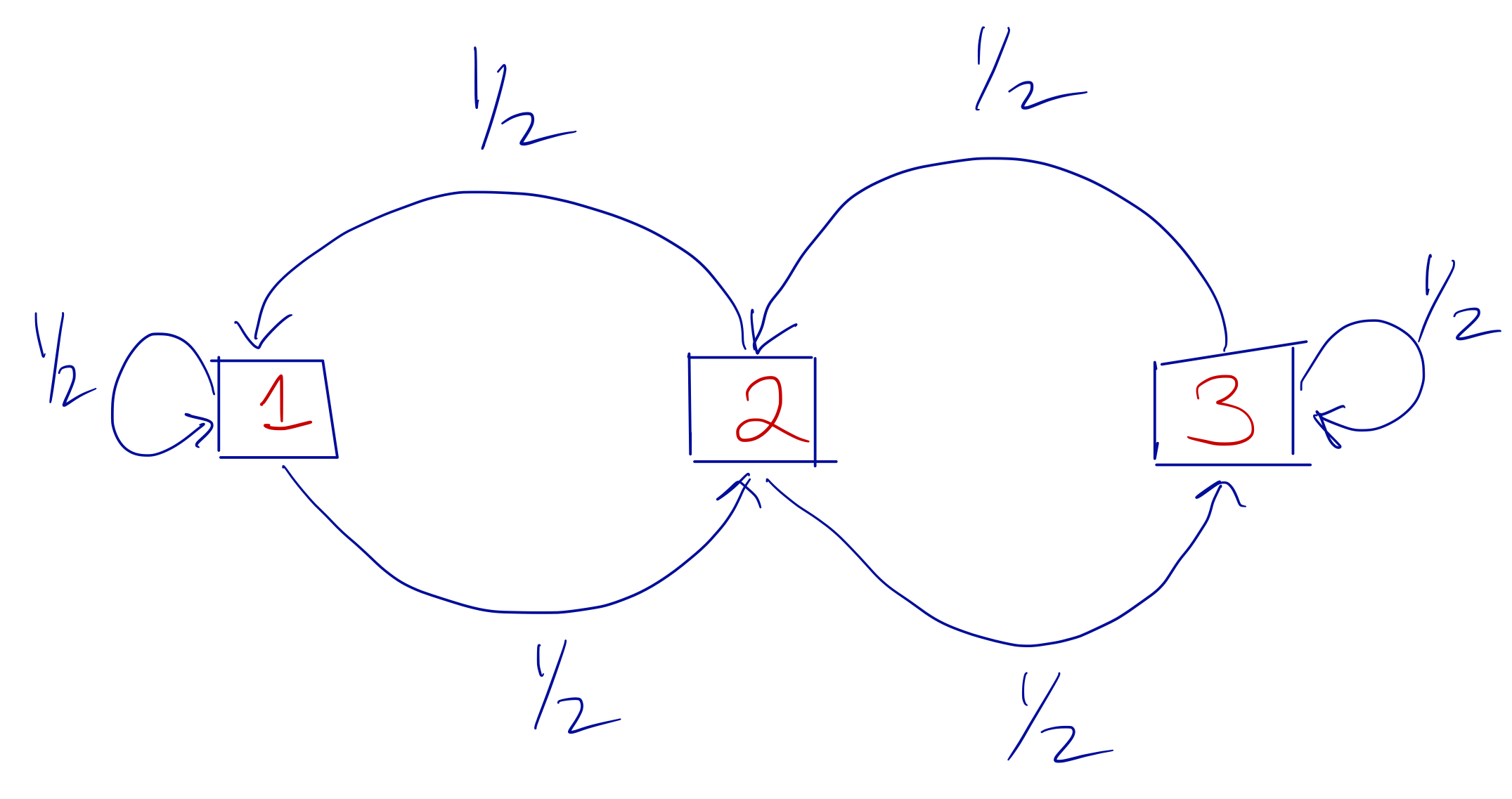
Simple Markov chain
Here, we have three states in the state space and the arrows indicate to which state you can travel given your current state. The fractions next to each arrow tell you what is the transition probabilities of going to a given state. Note that in this Markov chain, you can only ever travel to two possible states no matter what your current state happens to be.
We can write the transition probabilities in a matrix, a.k.a. the transition matrix, as \[ P = \left[ \begin{array}{ccc} 1/2 & 1/2 & 0\\ 1/2 & 0 & 1/2\\ 0 & 1/2 & 1/2 \end{array} \right] \] With the matrix notation, the interpretation of the entries is that if we are currently on interation \(n\) of the chain, then \[ \mathbb{P}(X_{n+1}=j\mid X_n=i) = P_{ij} \]
From the matrix, we can see that the probability of going from state \(1\) to state \(3\) is \(0\), because the \((1, 3)\) entry of the matrix is \(0\).
Suppose we start this Markov chain in state \(3\) with probability \(1\), so the initial probability distribution over the three states is \(\pi_0=(0,0,1)\). What is the probability distribution of the states after one iteration? The way the transition matrix works, we can write \[ \pi_1 = \pi_0 P = (0, 1/2, 1/2) \] A quick check of the diagram above confirms that if we start in state \(3\), then after one iteration we can only be in either state \(3\) or in state \(2\). So state \(1\) gets \(0\) probability.
What is the probability distribution over the states after \(n\) iterations? We can continue the process above to get \[ \pi_n = \pi_0 \overbrace{PPPP\cdots P}^{n\text{ times}} = P^{(n)} \] For example, after five iterations, starting in state \(3\), we would have \(\pi_5 = (0.3125, 0.34375, 0.34375)\).
7.1.2 Basic Limit Theorem
For a Markov chain with a discrete state space and transition matrix \(P\), let \(\pi_\star\) be such that \(\pi_\star P = \pi_\star\). Then \(\pi_\star\) is a stationary distribution of the Markov chain and the chain is said to be stationary if it reaches this distribution.
The basic limit theorem for Markov chains says that, under a specific set of assumptions that we will detail below, we have \[ \|\pi_\star - \pi_n\|\longrightarrow 0 \] as \(n\rightarrow\infty\), where \(\|\cdot\|\) is the total variation distance between the two densities. Therefore, no matter where we start the Markov chain (\(\pi_0\)), \(\pi_n\) will eventually approach the stationary distribution. Another way to think of this is that \[ \lim_{n\rightarrow\infty} \pi_n(i) = \pi_\star(i) \] for all states \(i\) in the state space.
There are three assumptions that we must make in order for the basic limit theorem to hold.
The stationary distribution \(\pi_\star\) exists.
The chain is irreducible. The basic idea with irreducibility is that there should be a path between any two states and that path should altogether have probability \(> 0\). This does not mean that you can transition to any state from any other state in one step. Rather, there is a sequence of steps that can be taken with positive probability that would connect any two states. Mathematically, we can write this as there exists some \(n\) such that \(\mathbb{P}(X_n = j\mid X_0 = i)\) for all \(i\) and \(j\) in the state space.
The chain is aperiodic. A chain is aperiodic if it does not make deterministic visits to a subset of the state space. For example, consider a Markov chain on the space of integers that starts at \(X_0=0\), and has a transition rule where \[ X_{n+1} = X_n + \varepsilon_n \] and \[ \varepsilon_n = \left\{ \begin{array}{cl} 1 & \text{w/prob } \frac{1}{2}\\ -1 & \text{w/prob } \frac{1}{2} \end{array} \right. \] This chain clearly visits the odd numbers when \(n\) is odd and the even numbers when \(n\) is even. Furthermore, if we are at any state \(i\), we cannot revisit state \(i\) except in a number of steps that is a multiple of \(2\). This chain therefore has a period of \(2\). If a chain has a period of \(1\) it is aperiodic (otherwise it is periodic).
7.1.3 Time Reversibility
A Markov chain is time reversible if \[ (X_0, X_1,\dots,X_n) \stackrel{D}{=} (X_n,X_{n-1},\dots,X_0). \] The sequence of states moving in the “forward” direction (with respect to time) is equal in distribution to the sequence of states moving in the “backward” direction. Further, the definition above implies that \((X_0, X_1)\stackrel{D}{=}(X_1,X_0)\), which further implies that \(X_0\stackrel{D}{=}X_1\). Because \(X_1\) is equal in distribution to \(X_0\), this implies that \(\pi_1=\pi_0\). However, because \(\pi_1=\pi_0 P\), where \(P\) is the transition matrix, this means that \(\pi_0\) is the stationary distribution, which we will now refer to as \(\pi\). Therefore, a time reversible Markov chain is stationary.
In addition to stationarity, the time reversibility property tells us that for all \(i\), \(j\), the following are all equivalent:
\[\begin{eqnarray*} (X_0, X_1) & \stackrel{D}{=} & (X_1, X_0)\\ \mathbb{P}(X_0=i, X_1=j) & = & \mathbb{P}(X_1=i, X_0 = j)\\ \mathbb{P}(X_0=i)\mathbb{P}(X_1=j\mid X_0=i) & = & \mathbb{P}(X_0=j)\mathbb{P}(X_1=i\mid X_0=j) \end{eqnarray*}\]
The last line can also be written as \[ \pi(i)P(i, j) = \pi(j)P(j, i) \] which are called the local balance equations. A key property that we will exploit later is that if the local balance equations hold for a transition matrix \(P\) and distribution \(\pi\), then \(\pi\) is the stationary distribution of a chain governed by the transition matrix \(P\).
Why is all this important? Time reversibility is relevant to analyses making use of Markov chain Monte Carlo because it allows us to find a way to construct a proper Markov chain from which to simulate. In most MCMC applications, we have no trouble identifying the stationary distribution. We already know the stationary distribution because it is usually a posterior density resulting from a complex Bayesian calculation. Our problem is that we cannot simulate from the distribution. So the problem is constructing a Markov chain that leads to a given stationary distribution.
Time reversibility gives us a way to construct a Markov chain that converges to a given stationary distribution. As long as we can show that a Markov chain with a given transition kernel/matrix satisfies the local balance equations with respect to the stationary distribution, we can know that the chain will converge to the stationary distribution.
7.1.4 Summary
To summarize what we have learned in this section, we have that
We want to sample from a complicated density \(\pi\).
We know that aperiodic and irreducible Markov chains with a stationary distribution \(\pi\) will eventually converge to that stationary distribution.
We know that if a Markov chain with transition matrix \(P\) is time reversibile with respect to \(\pi\) then \(\pi\) must be the stationary distribution of the Markov chain.
Given a chain governed by transition matrix \(P\), we can simulate it for a long time and eventually we will be simulating from \(\pi\).
That is the basic gist of MCMC techniques and I have given the briefest of introductions here. That said, in the next section we will discuss how to construct a proper Markov chain for simulating from the stationary distribution.