6 Results of empirical models
6.1 Ag
| Regionality test | ||
|---|---|---|
| Characteristic | Beta (95% CI)1 | p-value |
| log10(Rrs_665/Rrs_560) | 1.4 (1.3 to 1.5) | <0.001 |
| Region | ||
| EGSL | — | |
| JB | 0.00 (-0.05 to 0.05) | 0.93 |
| log10(Rrs_665/Rrs_560) * Region | ||
| log10(Rrs_665/Rrs_560) * JB | -0.23 (-0.43 to -0.03) | 0.026 |
|
1
CI = Confidence Interval
|
||
The Region parameter is not significant here, in fact, no real difference of trend are observed between the two regions.
Figure 6.1: Ag regionality
6.1.1 Ag(440)
Several band ratio model are presented hereafter.
The first one is fitted with a blue / red ratio. The blue part of the visible spectrum is the most influenced by CDOM absorption and it is expected to better grasp the variability according to the theory. In fact the distribution of \(a_g(440)\) with \(B(blue)/B(red)\) ratio is very sharp. It show a steep slope, likely induced by the saturation of light absorbed by CDOM as succinctly observed in 4.3 (see Figure 4.6) . There is a small constant offset between the measured and fitted value, the addition of a constant offset could then improve the model.
Figure 6.2: power law model for Ag, red over blue
| Characteristic | Beta (95% CI)1 | p-value |
|---|---|---|
| a | 3.4 (3.2 to 3.5) | <0.001 |
| b | 1.4 (1.3 to 1.5) | <0.001 |
|
1
CI = Confidence Interval
|
||
| MeanAE | MedAE | bias |
|---|---|---|
| 0.443 | 0.281 | 0.0883 |
| Region | rho |
|---|---|
| EGSL | -0.091 |
| JB | 0.170 |
The last one take advantage of of a green / red ratio, less affected by blue(ish) atmospheric correction errors and which give fairly good results. The slope of this distribution is less steep, confirming the saturation of light absorption by CDOM in the blue.
As this model present the least independents parameters and the best performance metrics it is chosen to be applied on Sensor images.
Figure 6.3: power law model for Ag, Red over Green
| Characteristic | Beta (95% CI)1 | p-value |
|---|---|---|
| a | 20 (17 to 24) | <0.001 |
| b | 1.8 (1.6 to 1.9) | <0.001 |
|
1
CI = Confidence Interval
|
||
| MeanAE | MedAE | bias |
|---|---|---|
| 0.344 | 0.233 | 0.0391 |
| Region | rho |
|---|---|
| EGSL | -0.01700 |
| JB | 0.00057 |
6.1.2 Houskeeper style
Figure 6.4: power law model for Ag, Red over Green
| Characteristic | Beta (95% CI)1 | p-value |
|---|---|---|
| a | 1.9 (1.8 to 2.1) | <0.001 |
| b | -0.45 (-0.49 to -0.41) | <0.001 |
|
1
CI = Confidence Interval
|
||
| MeanAE | MedAE | bias |
|---|---|---|
| 0.695 | 0.621 | 0.181 |
Figure 6.5: power law model for Ag, Red over Green
## [[1]]| MeanAE | MedAE | bias |
|---|---|---|
| 0.494 | 0.377 | 0.212 |
6.1.3 Ag(295, 275)
## [[1]]| MeanAE | MedAE | bias |
|---|---|---|
| 3.49 | 2.28 | 0.0159 |
## [[1]]| MeanAE | MedAE | bias |
|---|---|---|
| 4.76 | 3.42 | 0.152 |
6.1.4 Ag SPM relation
6.2 SPM
We try to see if the ‘Region’ variable created earlier is of any importance in the determination of \(C_{spm}\) from \(R_{rs}\) to do that we can use a generalized linear model, glm function in R. The formula that we used take the form \(SPM \sim Rrs(\lambda) + Region + Rrs(\lambda) * Region\) the last part of the formula express the interaction effect.
| Characteristic | Beta (95% CI)1 | p-value |
|---|---|---|
| log10(Rrs_665) | 0.29 (0.11 to 0.48) | 0.002 |
| Region | ||
| EGSL | — | |
| JB | 1.3 (0.69 to 2.0) | <0.001 |
| month(DateTime) | -0.05 (-0.08 to -0.03) | <0.001 |
| log10(Rrs_665) * Region | ||
| log10(Rrs_665) * JB | 0.63 (0.40 to 0.86) | <0.001 |
|
1
CI = Confidence Interval
|
||
As we see, \(R_{rs}\) and \(Region\) are significant variable to determine \(C_{spm}\), \(C_{spm}\) varies both across \(R_{rs}\) and \(Region\). The interaction factor is also significant, meaning that \(C_{spm}\) relation with \(R_{rs}\) also varies with \(Region\).
What could be misleading here, is that \(C_{spm}\) varying across \(Region\) is also a matter of \(C_{spm}\) range. This one is wider for JB than for EGSL, hence it may affect the significance of \(Region\).
Considering the results presented above, models have been fitted specifically for those region.
Grouped under the Estuary and Gulf of Saint-Lawrence (EGSL) and James Bay (JB) region, distribution of \(C_{spm}\) vs \(R_{rs}\) show two clear and different pattern.
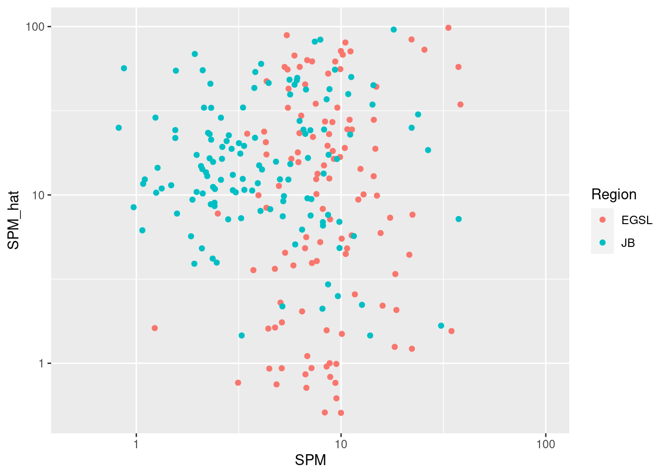
6.2.1 SPM from Rrs
| Characteristic | EGSL | JB | ||
|---|---|---|---|---|
| Beta (95% CI)1 | p-value | Beta (95% CI)1 | p-value | |
| a | 3.6 (2.0 to 6.5) | <0.001 | 13 (8.7 to 19) | <0.001 |
| b | 0.21 (0.13 to 0.30) | <0.001 | 0.52 (0.44 to 0.60) | <0.001 |
|
1
CI = Confidence Interval
|
||||
| Region | MeanAE | MedAE | bias |
|---|---|---|---|
| EGSL | 3.42 | 1.790 | 0.518 |
| JB | 3.47 | 0.829 | 0.296 |
| Region | rho |
|---|---|
| EGSL | c(S = 808886), NULL, 0.00845479915636648, c(rho = 0.194922820137927), c(rho = 0), two.sided, Spearman's rank correlation rho, Ag_440 and SPM - (10^pred) |
| JB | c(S = 297785.219727441), NULL, 4.00762873935923e-12, c(rho = 0.520181077426701), c(rho = 0), two.sided, Spearman's rank correlation rho, Ag_440 and SPM - (10^pred) |
6.2.2 Test
6.2.3 SPM from Rrs_740
| Characteristic | EGSL | JB | ||
|---|---|---|---|---|
| Beta (95% CI)1 | p-value | Beta (95% CI)1 | p-value | |
| a | 3.8 (2.2 to 6.6) | <0.001 | 17 (12 to 23) | <0.001 |
| b | 0.19 (0.12 to 0.27) | <0.001 | 0.42 (0.38 to 0.47) | <0.001 |
|
1
CI = Confidence Interval
|
||||
| Region | MeanAE | MedAE | bias |
|---|---|---|---|
| EGSL | 3.34 | 1.820 | 0.649 |
| JB | 1.86 | 0.875 | 0.201 |
6.2.4 SPM 560
| Characteristic | EGSL | JB | ||
|---|---|---|---|---|
| Beta (95% CI)1 | p-value | Beta (95% CI)1 | p-value | |
| a | 3.8 (2.2 to 6.6) | <0.001 | 17 (12 to 23) | <0.001 |
| b | 0.19 (0.12 to 0.27) | <0.001 | 0.42 (0.38 to 0.47) | <0.001 |
|
1
CI = Confidence Interval
|
||||
| Region | MeanAE | MedAE | bias |
|---|---|---|---|
| EGSL | 3.90 | 1.76 | 0.517 |
| JB | 4.75 | 1.71 | 1.020 |
6.2.5 SPM Moham
| Coefficient for Rrs(710)/Rrs(665) | ||||
|---|---|---|---|---|
| Characteristic | EGSL | JB | ||
| Beta (95% CI)1 | p-value | Beta (95% CI)1 | p-value | |
| a | 14 (9.9 to 19) | <0.001 | 38 (31 to 44) | <0.001 |
| b | 1.0 (0.26 to 1.7) | 0.009 | 4.0 (3.3 to 4.9) | <0.001 |
|
1
CI = Confidence Interval
|
||||
| Region | MeanAE | MedAE | bias |
|---|---|---|---|
| EGSL | 4.31 | 3.04 | 2.44 |
| JB | 7.22 | 3.3 | 2.33 |
6.2.6 SPM from Bbp_532
| Characteristic | Beta (95% CI)1 | p-value |
|---|---|---|
| log10(Bbp_532) | 0.27 (0.12 to 0.43) | <0.001 |
| Region | ||
| EGSL | — | |
| JB | 0.27 (-0.06 to 0.61) | 0.11 |
| log10(Bbp_532) * Region | ||
| log10(Bbp_532) * JB | 0.56 (0.36 to 0.76) | <0.001 |
|
1
CI = Confidence Interval
|
||
Regionality is strongly confirmed in the relation SPM ~ Bbp(532)
| Coefficient of linear model | ||||
|---|---|---|---|---|
| Characteristic | EGSL | JB | ||
| Beta (95% CI)1 | p-value | Beta (95% CI)1 | p-value | |
| (Intercept) | 1.4 (1.1 to 1.7) | <0.001 | 1.7 (1.5 to 1.8) | <0.001 |
| log10(Bbp_532) | 0.27 (0.10 to 0.45) | 0.002 | 0.83 (0.72 to 1.0) | <0.001 |
|
1
CI = Confidence Interval
|
||||
| Region | MeanAE | MedAE | bias |
|---|---|---|---|
| EGSL | 4.20 | 2.030 | -0.525 |
| JB | 3.35 | 0.715 | 0.398 |
6.2.7 Bbp_532 from Rrs
Theoretically IOPs are not region specific and could be retrieved from AOPs with a single model. If this hold true, retrieving Bbp from Rrs and then linking Bbp to Cspm could improve Cspm retrieval from space.
| Characteristic | Beta (95% CI)1 | p-value |
|---|---|---|
| log10(Rrs_665) | 1.0 (0.89 to 1.2) | <0.001 |
| Region | ||
| EGSL | — | |
| JB | -0.19 (-0.69 to 0.32) | 0.47 |
| log10(Rrs_665) * Region | ||
| log10(Rrs_665) * JB | -0.17 (-0.35 to 0.01) | 0.074 |
|
1
CI = Confidence Interval
|
||
In fact, regionality is not conclusive for Bbp in our dataset.
Figure 6.6: Bbp(532) from MSI Rrs(664.6)
However, a closer look at the distribution seems to indicate an offset, notably in lower values.