4 Exploratory data analysis
4.1 Spectrum plot
It’s always nice to start a study on remote sensing with the spectrum plot of in-situ data. The spectrum shown here are simulated for MSI. To improve the information they carry, each spectrum is colored by its associated concentration of CDOM or SPM (should be able to switch that with a button in plotly). To add some more fun, the sliders enable to filter both plots by those concentration.
Figure 4.1: Effect of SPM concentration on Rrs spectrum
Figure 4.2: Effect of CDOM absorption on Rrs spectrum
4.2 Summary stats
4.2.1 Density of reflectances
All reflectance distribution are heavily skewed toward lower intensities. This need to be taken into account in the statistic used has assumptions will break down. Deselect everything and then add the band one by one, you will see that maximum of the variability is observed between 500 and 700 nm (B2 to B5). Yet a smaller but significant amount of this variability is observed in band B1, B6, B7.
Figure 4.3: Density plot of remote sensing reflectance as seen by MSI, for EGSL and JB
##
-
\
../../sandbox/linux/seccomp-bpf-helpers/sigsys_handlers.cc:**CRASHING**:seccomp-bpf failure in syscall 0230
##
|
/
../../sandbox/linux/seccomp-bpf-helpers/sigsys_handlers.cc:**CRASHING**:seccomp-bpf failure in syscall 0230
##
-
\
../../sandbox/linux/seccomp-bpf-helpers/sigsys_handlers.cc:**CRASHING**:seccomp-bpf failure in syscall 0230
##
|
/
-
\
|
Summary statistic are given here for the entire dataset, meaning that it’s before outlier removal and there is incomplete cases of \(R_{rs}\) with \(C_{spm}\) and \(a_g(440,295,275)\). To be exact about model validity range, summary stats of \(C_{spm}\) and \(a_g\), train and test dataset are given.
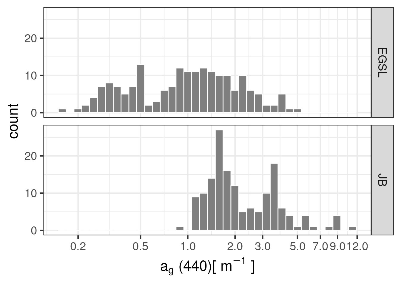
4.2.2 Distribution of SPM and CDOM
Absorption by CDOM at 440 nm (\(a_g(440)\), g for gelbstoff from German “yellow substance”) is used as a proxy for CDOM concentration
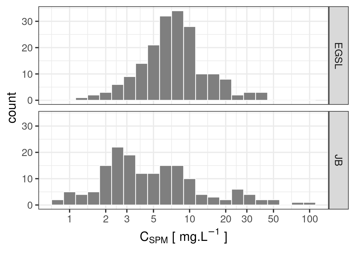
This section intend to explore and explain the physical basis allowing empirical models to grasp the natural variability of OACs, hence retrieving their concentration from water color.
4.3 Ag spectrum with sensors bands
It is shown in Gitelson et al (1993) that empirical model based on band arithmetic, specifically band ratio, have the ability to retrieve concentration of OACs. The logic of the band ratio model is to select two band, one “active” sensitive to the target OAC and one “reference” nonsensitive. The division of the sensitive band by the nonsensitive act as a normalization function.
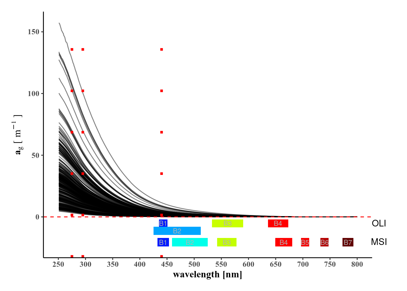
Figure 4.4: Absorption spectrum of CDOM with OLI and MSI bandwidth, red line represent retrival target wavelength of Ag
The principal difficulty in this approach is the overlap in IOPs spectrum of different constituents. See IOPs in this database dashboard to get a better sense of it. First selecting the IOPs of interest, then selecting a station (click on row) in the table will highlight corresponding IOPs spectrum. By deselecting the trace in first step, only the selected row(s) will remain and axis range will update accordingly.
It is particularly interesting to compare CHONE_216 and PMZA-RIKI_004 to highlight difference of water type between coastal station and in the middle of the St-Lawrence.
When comparing the distribution in log space of \(a_g\) with \(R_{rs}\) from MSI band 1 to 6, we see a shift in the relation. Negative in the blue, null in the green and positive in the red.
Figure 4.5: Ag(440) and Rrs as seen by MSI bands (colored by Project)
Colored by SPM, it indicate events of high SPM and CDOM concentration occurring simultaneously.
| Bbp Ag coeff | ||||
|---|---|---|---|---|
| Characteristic | EGSL | JB | ||
| Beta (95% CI)1 | p-value | Beta (95% CI)1 | p-value | |
| (Intercept) | -2.1 (-2.5 to -1.7) | <0.001 | -1.7 (-1.8 to -1.5) | <0.001 |
| log10(Ag_532) | 0.03 (-0.54 to 0.61) | 0.91 | 0.48 (0.12 to 0.85) | 0.010 |
| log10(SPM) | 0.46 (0.02 to 0.90) | 0.040 | 0.73 (0.59 to 0.87) | <0.001 |
| log10(Ag_532) * log10(SPM) | 0.29 (-0.33 to 0.90) | 0.36 | -0.52 (-0.91 to -0.13) | 0.009 |
|
1
CI = Confidence Interval
|
||||
## # A tibble: 2 × 2
## Region r2
## <chr> <dbl>
## 1 EGSL 0.539
## 2 JB 0.668## # A tibble: 2 × 3
## Region r2 pvalue
## <chr> <dbl> <dbl>
## 1 EGSL 0.503 8.87e-10
## 2 JB 0.391 1.91e- 6## # A tibble: 2 × 2
## Region r2
## <chr> <dbl>
## 1 EGSL 0.335
## 2 JB 0.455##
-
\
../../sandbox/linux/seccomp-bpf-helpers/sigsys_handlers.cc:**CRASHING**:seccomp-bpf failure in syscall 0230
##
|
/
../../sandbox/linux/seccomp-bpf-helpers/sigsys_handlers.cc:**CRASHING**:seccomp-bpf failure in syscall 0230
##
-
\
../../sandbox/linux/seccomp-bpf-helpers/sigsys_handlers.cc:**CRASHING**:seccomp-bpf failure in syscall 0230
##
|
/
-
\
|
## # A tibble: 2 × 2
## Region mean_Ag665
## <chr> <dbl>
## 1 EGSL 0.0288
## 2 JB 0.0549How to investigate the nonuniqueness problem (ambiguity) ?
-Define range slider for quantities of interest -Define discrete colors by range
Outside the log space, a saturation point is observed near a value of 3 \(a_g\). Considering that \(Ed0^+\) is a finite power incident to the water surface (\(\phi_i\)), with \(\lim_{\phi_a \to \phi_i}f(R_{rs}) = 0\)
Figure 4.6: Saturation effect in Rrs(blue) by Ag
Saturation seem to occur near \(4\ a_g(440)[m^{-1}]\) according to a log linear model (fitted black line). I need to find a mathematical approach to define this.
SPM is linked to the Rrs signal through Bbp and Ap, regional specificity in the mass specific absortion and scatering of SPM change the magnitude of these relation.
4.4 Interrelation of OACs/IOPs with \(R_{rs}\)
Figure 4.7: SPM vs Rrs colored by CDOM
Figure 4.8: Bbp vs Rrs colored by CDOM
Figure 4.9: CDOM vs Rrs colored by SPM
| Spearman rho | |
|---|---|
| for C<sub>SPM</sub> and R<sub>rs</sub>(665,740) | |
| Region | r2 |
| EGSL | 0.3974803 |
| JB | 0.8052560 |
SPM and CDOM concentration seems to some extension to be positively covariant in James Bay. As \(C_{spm}\) increase, \(a_g(440)\) also increase. This graph is insightful on the mixing EGSL and James Bay distribution.
Figure 4.10: SPM vs Rrs(550) colored by Ag(440)
SPM and Bbp confirm the observed regional Rrs SPM pattern.
Figure 4.11: SPM vs Bbp
Two clusters emerges when comparing JB \(b_{bp}^\star SPM\) vs \(b_{bp}^\star PIM\)
##
-
\
|
../../sandbox/linux/seccomp-bpf-helpers/sigsys_handlers.cc:**CRASHING**:seccomp-bpf failure in syscall 0230
##
/
-
../../sandbox/linux/seccomp-bpf-helpers/sigsys_handlers.cc:**CRASHING**:seccomp-bpf failure in syscall 0230
##
\
|
/
../../sandbox/linux/seccomp-bpf-helpers/sigsys_handlers.cc:**CRASHING**:seccomp-bpf failure in syscall 0230
##
-
\
|
/
| Region | bbp | ap |
|---|---|---|
| EGSL | 0.018 | 0.23 |
| JB | 0.078 | 0.34 |
| Region | Ag440 | SPM | bbp | ap | bbp*SPM | bbp*PIM | ap*SPM |
|---|---|---|---|---|---|---|---|
| EGSL | 1.3 | 9.0 | 0.018 | 0.23 | 0.0021 | 0.0027 | 0.032 |
| JB | 2.6 | 8.5 | 0.078 | 0.34 | 0.0140 | 0.0170 | 0.083 |
Bbp spectrum likely have different regional shape as indicated by Rrs as 740 nm
This confirm that IOPs are not region dependent, a single models retrieving Bbp could be used to then retrieve SPM from Bbp.
Figure 4.12: Bbp532 vs Rrs(664.6)
SPM vs Bbp and Rrs are in good agreement.
4.4.1 SPMs assemblage
Figure 4.13: SPM vs Bbp(532) colored by PIM/SPM fraction
Coast JB data seem unreliable with PIM > SPM … cleaning would be needed.
4.4.2 Bottom effect
The Secchi depth \([m^{-1}]\) is a measure of light penetrability in the water column. It’s made with a disk (Secchi disk) divided in black and withe quarter. When the disk disappear in the depth, it mean that the light cannot reach it and come back to our eye. The Secchi depth is taken at that point, since the light have to cross back and forth the water column we may assume that it reaches two time the Secchi depth. This assumption is used here to determine the measurement made in optically shallow water. Bottom effect are assumed when \(Zsecchi . 2 > Zstation\) or \(Zsecchi = 999\) (Secchi disk touch the bottom). However, here we also assume that light travel in the water and at the air/water interface with linearity, which break down according to Beer-Lambert law. No conclusive result is taken from this method.
Figure 4.14: Identification of optically shalow waters acording to the linear formula: Zsecchi . 2 > Zstation
4.4.3 SPM Depth Covariance
Resuspension may be attributed to shallow water waves, \(Depth <= \frac{\lambda_{wave}}{2}\) which would explain highest Cspm measured in shallow waters. This is particularly clear for the shallow waters of Jame Bay. Data on wave and/or wind speed and direction would be necessary to dig this.
Figure 4.15: SPM depth covariance attributed to resuspension
4.4.4 SPM and reflectance depandance on month of sampling
Figure 4.16: Identification of data point quality check by region