Chapter 4 Model Structures
Based on related theories and studies, this section introduces several different analytical frameworks. Götschi et al. (2017) analyses the frameworks of 26 studies on active travel behavior. They propose a conceptual framework covering physical and social determinants, individual and multi-spatial levels. The three explanatory frameworks introduced in this section can find supportive evidences and reflect the cognitive differences on travel-urban form studies. This section does not intend to figure out a ‘best’ framework. It demonstrates the structures from various perspectives would lead to distinct models and results.
4.1 Multistage
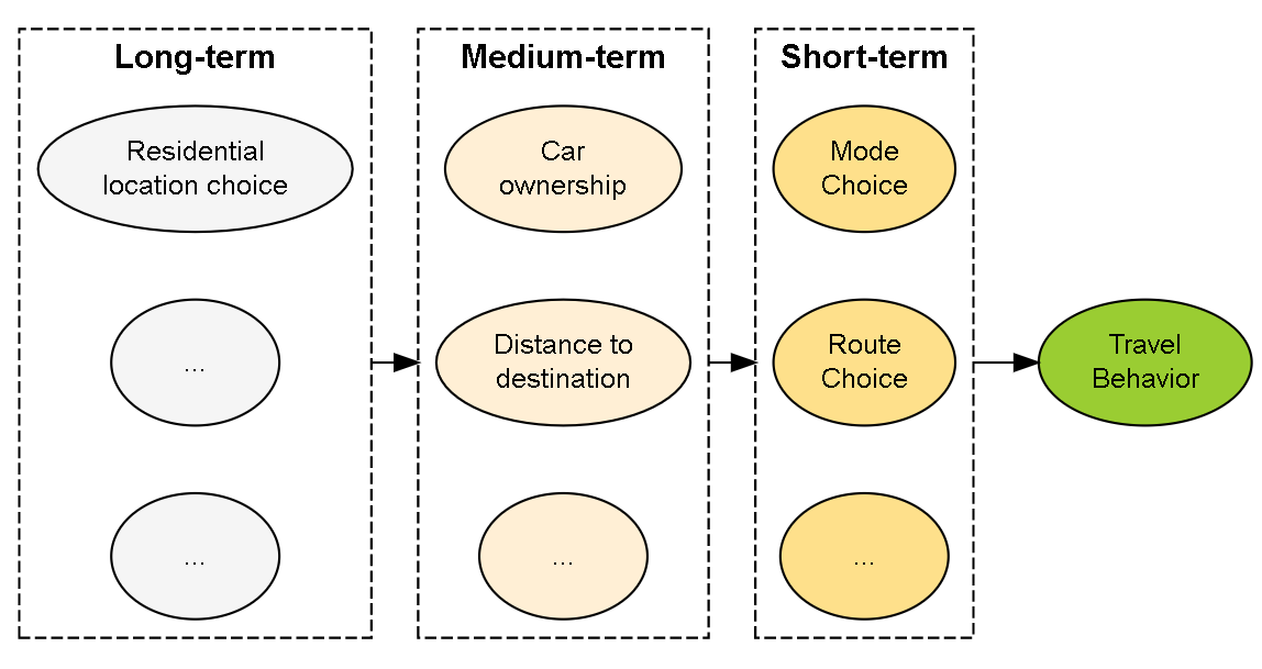
Figure 4.1: Multistage Structure
Ben-Ariva and Atherton (1977) introduced a hierarchical framework of travel behavior. According to the length of time in travel decision, they divided the relevant factors into three levels. For example, people could change their travel mode choice for each day or each trip. Thus mode choice is a short-term decision Car ownership belongs medium-term decision since people usually don’t purchase or sell a car very often. Residential location choice is long-term decision because relocation is the most infrequent event than others.
Under this framework, the decisions in longer term can affect the decisions in shorter term, but not vice versa. (Figure 4.1) For example, the distance to destination is decided by residential location choice and working location choice. And the distance is also a fundamental factor that influences travel mode choice behavior (Munshi 2016). In this way, both household car ownership, travel distance and travel attitudes are treated as intermediate variables connecting between built environment and mode choice in decision models. (Ding, Wang, et al. 2017; De Vos et al. 2021). A VMT models with stepwise framework is as follow.
\[\begin{equation} \tag{4.1} \mathrm{Y}=\mathbf{X}_\mathrm{L}\boldsymbol{\beta}_\mathrm{L}+\mathrm{X_{M}}{\beta}_\mathrm{M}+\mathbf{X}_\mathrm{S}\boldsymbol{\beta}_\mathrm{S}+\boldsymbol{\varepsilon} \end{equation}\]
where \(\boldsymbol{\beta}\) are the coefficients with respect to long-term factors \(\mathbf{X}_\mathrm{L}\), medium-term \(\mathrm{X_{M}}\), and short-term covariates \(\mathbf{X}_\mathrm{S}\). There could be two-way interaction effect between long-term and medium-term variables; three-way interaction effects among long-term, medium-term and short-term variables in the model (Equation (4.1)).
This framework works well for commuting trips because people will not change work place very often. The mobility theories also agree with this pattern. “commuting trips are stable in time and account for the largest fraction of the total flows in a population.” (Van Acker and Witlox 2011).
However, the number of weekdays commute trips in the U.S. are less than one third of total trips in many years (source: U.S. Department of Transportation, Federal Highway Administration 2009). For non-work travel purposes, such as shopping, leisure, or socializing, the destination choices are more flexible.
The decision could be one-step. In consideration of all the benefit and cost, The traveler make a decision including the destination, mode and route at the same moment. It also could be multistep. Starting from a travel demand or purpose, the traveler decides to make a trip then choose the destination, mode, route, and departure time step-by-step from available alternatives based on benefit, cost, and habit. This process is progressive, iterative, and habitual in real life. Hence, the travel distance could be decided before or after mode or route choices. One structure only can capture one aspect of the process. The framework selection should suit the research question.
4.2 Decision Tree
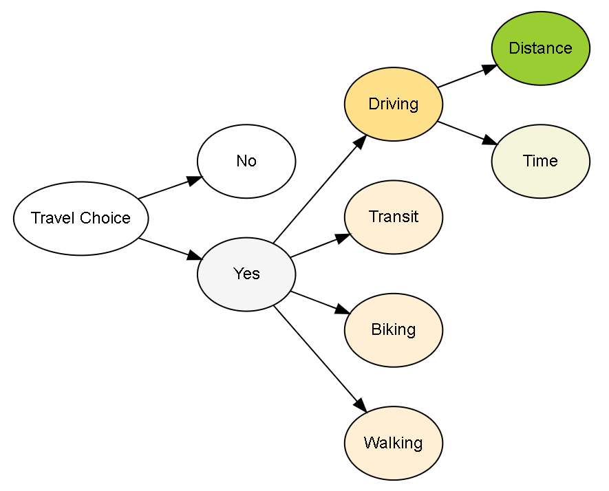
Figure 4.2: Decision Tree Structure
The single-step decision frameworks often require some strong assumptions. For example, the principle of utility maximization applied in either mode choice or VMT models is supposed to explain all the observations, including no-trip or no-driving cases. Here these observation are treated as censored data with negative utilities. (That will leads to Tobit model for VMT.)
In contrast, a Decision Tree structure allows to use a hierarchical structure to fit different observation respectively (Figure 4.2). A similar figure can be found in Reid Ewing et al. (2011) ’s Figure .1. This structure is suitable for the studies including both mode choice and distance/time variables (Ma, Yan, and Weng 2015; Reid Ewing et al. 2015). The model will split into three equations (4.2) Starting from a travel demand or purpose, the traveler decides to make a trip or not at the first-level dichotomous node. A logit or probit model will fit all the data using a suitable model specification.
Then the second layer with polychotomous nodes is about mode choice, which is respect to the multinomial models. At the bottom layer, a linear (or log-linear) model will only fit the data with positive driving distance (hurdle models; Ma, Yan, and Weng (2015); Reid Ewing et al. (2015)). It is remarkable that the covariates set could vary in different layer’s models. For example the lifecycle factor could strongly affect the travel frequency but not affect the driving distance significantly. Therefore, this structure is more flexible and is consistent with real decision process.
\[\begin{equation} \begin{split} E[\mathbf{Y}_{\{yes,no\}}|\mathbf{X_0}]=&\boldsymbol{\mu_0}=g^{-1}(\mathbf{X_0}\boldsymbol{\beta})\\ E[\mathbf{Y}_{\{car,bus,...\}}|\mathbf{X_1},\mathbf{Y}_{\{yes\}}]=&\boldsymbol{\mu_1}=g^{-1}(\mathbf{X_1}\boldsymbol{\gamma})\\ \mathbf{Z}_{\{car\}}=&\mathbf{X}_\mathrm{2}\boldsymbol{\delta} + \boldsymbol{\varepsilon} \end{split} \tag{4.2} \end{equation}\]
where \(\mathbf{Y}_{\{yes,no\}}\) is a binary variable of making a trip or not. \(\mathbf{Y}_{\{car,bus,...\}}\) is a categorical variable only including the cases of making a trip. \(\mathbf{Z}_{\{car\}}\) is a continuous variable represent driving distance among the group of choosing driving. \(\mathbf{X}_{\{0,1,2\}}\) means the three equations could have different model specifications and will estimate corresponding coefficients, \(\boldsymbol{\beta}\), \(\boldsymbol{\gamma}\), and \(\boldsymbol{\delta}\).
4.3 Multi-scales
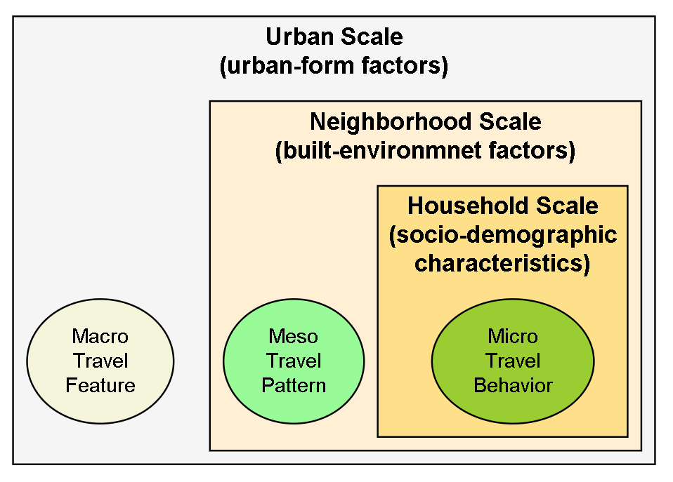
Figure 4.3: Multi-scales Structure
As discussed in previous section, the external factors affect individual’s travel behavior at multiple scales (Figure 4.3). This structure is adapted by many studies in recent years (Reid Ewing et al. 2011, fig. 3). Multi-scales studies distinguish the micro-, meso, and macro-scale variables (Ding, Mishra, et al. 2017; S. Lee and Lee 2020). According the results, Van Dender and Clever (2013) doubt whether VMT is determined by local built environment factors. The external factors always affect a group of individuals. Therefore, the meso-scale factors like built environment still can be examined. But the social and nature environment will impact all the people living inside the cities and regions. Only when the data sources cover many cities or regions, these factors can be involved in the models.(Equation (4.3))
\[\begin{equation} \tag{4.3} \mathbf{Y}=\mathbf{X}_\mathrm{U}\boldsymbol{\beta}_\mathrm{U}+\mathbf{X}_\mathrm{N}{\beta}_\mathrm{N}+\mathbf{X}_\mathrm{H}{\beta}_\mathrm{H}+\cdots+\boldsymbol{\varepsilon} \end{equation}\]
where \(\mathbf{X}_\mathrm{U}\), \(\mathbf{X}_\mathrm{N}\), and \(\mathbf{X}_\mathrm{H}\) are the covariates at the scales of urban, neighborhood, and household. And \(\boldsymbol{\beta}_\mathrm{U}\), \(\boldsymbol{\beta}_\mathrm{N}\), and \(\boldsymbol{\beta}_\mathrm{H}\) are corresponding coefficients respectively.
4.4 Other Structures
- Mixed Model
Regression models usually assume the fixed effects of covariate on response. In many cases, some variables should be assigned with random effects. In travel survey data, every observation are nested in some geographic units, such as tract, TAZ, or city (Ding, Mishra, et al. 2017). The geographic location often have some nature of artificial feature influencing travel but the factor is unknown or unobserved. When the data across many different regions, the model need to control the location effect to identify the crossed effect of built environment. For example, the hypothesis is whether density variable has a strong effects on travel in all place.
In spatial analysis, autocorrelation is a common issue which means the observation values in a location will be affected by its neighbors. Mixed model can help to eliminate the neighborhood effects.
\[\begin{equation} \tag{4.3} \mathbf{Y}=\mathbf{X}_\mathrm{H}\boldsymbol{\beta}+\mathbf{X}_\mathrm{N}{\gamma}+\mathbf{X}_\mathrm{U}{\delta}+\boldsymbol{\varepsilon} \end{equation}\]
where \(\mathbf{X}_\mathrm{U}\), \(\mathbf{X}_\mathrm{N}\), and \(\mathbf{X}_\mathrm{H}\) are the same as above. \(\boldsymbol{\beta}\) is a vector of fixed effects. \(\boldsymbol{\gamma}\) and \(\boldsymbol{\delta}\) are two vectors of random effects at neighborhood and urban scales. Assume that \(\boldsymbol{\gamma}\sim N(\mathbf{0}, \boldsymbol{\Sigma}_\mathrm{N})\) and \(\boldsymbol{\delta}\sim N(\mathbf{0}, \boldsymbol{\Sigma}_\mathrm{U})\). And also assume \(Cov(\boldsymbol{\gamma},\boldsymbol{\delta})=Cov(\boldsymbol{\gamma},\boldsymbol{\varepsilon})=Cov(\boldsymbol{\delta},\boldsymbol{\varepsilon})=\mathbf{0}\).
- Non-linear models
As Clifton (2017) said, built environment-travel studies often assume the linearity holds for the density measures and the travel outcome of interest. In practice, the relationship of trip vesus built environment variables may be non-linear or follow a step function with lower and upper threshold. The shape of the curve is highly informative. Recently, scholars have an increasing interest in the non-parameter methods (Ding et al. 2021). The overall effects of density might be small. But the curve might have a steep rise or sheer drop in some intervals. The inflection points, called effective thresholds, are more attractive and instructional. For example, Using Generalized Additive Model (GAM) (Hastie and Tibshirani 1990), Reid Ewing et al. (2020) ’s study finds some potential points of encouraging shorter driving. His study recommended the suitable activity density (population and employment size/square mile) should be between 10000-25000 according to a center type (Figure ). More and more studies reveal the non-linear relationship between population density and VMT (Cheng et al. 2020; Ding, Cao, and Næss 2018). People can interpret the different trends as trigger effects, ceiling effects, U-shapes, hybrid, or synergy effect.
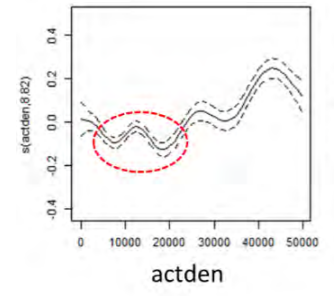
Figure 4.4: Activity density v.s its smooth function ( Source: Ewing, R. 2021. Webinar: Transportation Benefits of Polycentric Urban Form)
\[\begin{equation} \tag{4.4} \mathrm{Y}=\mathbf{X}_\mathrm{C}\boldsymbol{\beta}_\mathrm{C}+m(\mathbf{X}_\mathrm{E})\boldsymbol{\beta}_\mathrm{E}+\boldsymbol{\varepsilon} \end{equation}\]
In the model (Equation (4.4)), \(m(\mathbf{X}_\mathrm{E})\) is a proper function of built environment covariates.
The non-linear methods can better perform goodness-of-fit, but the generated new data are unique and harder to interpret. The non-linear methods can disclose more information from the data. The risk is that their results are more likely to reflect the features of the data itself and cannot be generalized to other cases.
The results of linear and non-linear models cannot be compared because their underlying assumptions of distribution are different. The threshold studies in urban transportation field remain in the early stages.