Chapter 7 Several Issues
This chapter goes through several common issues in modeling and discuss the potential risks and remedies. Ignoring these issues could lead to severe biased estimates or spurious relationships. In a travel-urban form paper, the part of methodology usually includes data, variables, models, and results. Before publication, the researcher must have done a lot of work: trying any possible data sources, conducting variable selection and completing model validation. These works often are not shown in the paper. Therefore, the topics in this chapter are potential issues. A suitable literature review or convincing criticism requires to gather the original data and replicate the models in the published paper.
7.1 Assumptions
- Additive and linearity
For regression models, relationship between the explanatory variables should be additive. The initial relationship could be multiplicative or exponential. log transform can covert the multiplicative relationship to additive (Choi et al. 2012). The proper specification requires some theoretical and empirical supports. Gravity Law discloses that travel distance has a multiplicative (inverse) relationship with the ‘masses’ of two places. The ‘masses’ related variable such as population size can be added to the regression model as a additive factor.
Some built environment and socioeconomic factors may have interaction effects. For example, the high density in developed countries have different effects on travel to the developing countries (Reid Ewing and Cervero 2017). Exploring the two-way or even higher order interaction effects is not common in travel-urban form studies. S. Lee and Lee (2020) examine the interaction effects between population weighted density (PWD) and D-variables at tract level. Other possible paired interactions are not considered in this study.
Linearity means the function of independent variables is compatible with addition and scaling. That is \(f(x+y)=f(x)+f(y)\) and \(f(a\cdot x)=a\cdot f(x)\). When the assumption of linearity still doesn’t hold after transformation, the study should look for other non-linear models and corresponding approaches. Does the regression models show the linear property after log transformation? There are more recent studies start to pay attention to this topic (Reid Ewing et al. 2020; Ding et al. 2021). More discussion of the non-linear relationship is placed in the next chapter.
- Independent Identically Distributed (IID)
Another essential assumption is that random error are Independent Identically Distributed (IID). Random error is also called residual, which refer to the difference between observed \(\mathbf{y}\) and fitted \(\mathbf{\hat y}\). That is \(\mathbf{e}=\mathbf{y}-\mathbf{\hat y}\), where \(\mathbf{\hat y}\) are the linear combinations of predictors \(\mathbf{X}\). Residuals represent the part can not be explained by the model.
‘Identical’ means that random errors should have zero mean and constant variance. The expected value, the variances, and the covariances among the random errors are the first- and second-moment of residuals. That is \(E(\varepsilon) = 0\) and \(Var(\varepsilon) = \sigma^2\). The homogeneity of variance is also called homoscedasticity. To satisfy this assumption, some studies chose a subset such as VMT by nonwork purposes (Chatman 2008), bus ridership by time of day, or school children’s metro ridership (Liu et al. 2018). So it also depends on the research design.
‘Independent’ requires the random errors are uncorrelated. That is \(Cov[\varepsilon_i,\varepsilon_j] = 0\),\(i\neq j\) In the stage of survey design, researchers try to collect the data by random sampling. The studies using secondary data usually believe every observations are independent. But in travel-urban form studies, many dataset cover all the neighbored units in a region. In this situation, the independent assumption often doesn’t hold.
- Normality
The common words in travel-urban form literature are that “We use logarithm transform on travel variables to address the issues of normality and linearity.” Evidence has demonstrated that travel distance and frequency are not Normal distributed. The Zipf’s law also prove that travel distance follows a power distribution. Using logarithm transformations, the skewed distribution can be converted to an approximate normal distribution. Meanwhile, some scholars assume the observed travel data are left censored and choose Tobit regression (Chatman 2003; M. G. Boarnet, Greenwald, and McMillan 2008).
Actually, the normality requirement for response is a misunderstanding. Neither response variable nor predictor is required to be normal. Normality is the requirement for residuals. Note that least squares method itself needs zero mean and constant variance rather than normality. When conducting hypothesis test and infering confidence intervals, the required assumption is that the response conditional on covariates is normal, that is \(\mathbf{y|x}\sim N (\mathbf{X}\boldsymbol{\beta},\sigma^2\mathbf{I})\). Maximum Likelihood Methods also requires this assumption. There are some quantitative methods which can examine normality of the transformed distributions.
- A brief Discussion
In urban studies, the geographic data often have both independent and identical issues, which are called the spatial autocorrelation and heterogeneity (Lianjun Zhang, Ma, and Guo 2009). That means, the observation in one location be affected by the neighbored areas for some unknown reasons. And the observations from city to city or region to region are generated by distinct mechanisms. Once the conditions of IID are satisfied, the Gauss - Markov theorem proves that least-square method could give the minimum-variance unbiased estimators (MVUE) or called the best linear unbiased estimators (BLUE). These conditions are not strict and make regression method widely applicable.
When the sample size is small, the circumstance of violating normality assumption would make the inference misleading. As Lumley et al. (2002) pointed out, if the sample size is large enough such as \(n\ge 100\), the t-test and OLS still can give the asymptotically unbiased estimates of mean. But for some long-tailed data, median regressions might be appropriate, that also depends on the research question to be asked. Few paper in travel-urban form literature show their normality test in the published version and investigate the influences.
7.2 Adequacy
The estimation and inference themselves can not demonstrate a model’s performance. If the primary assumptions is violated, the estimations could be biased and the model could be misleading. These problems can also happen when the model is not correctly specified. Making a proper diagnosis and validation are the first thing we need to do when fitting some models.
- Residuals Analysis
The major assumptions, both IID and normality are related to residual. Residual diagnosis is an essential step for modeling validation. There are several scaled residuals can help the diagnosis. Since \(MSE\) is the expected variance of error \(\hat\sigma^2\) and \(E[\varepsilon]=0\), standardized residuals (\(d_i=\frac{e_i}{\sqrt{MSE}}=e_i\sqrt{\frac{n-p}{\sum_{i=1}^n e_i^2}}\), \(i=1,2,...,n\)) should follow a standard normal distribution.
Recall random error \(\mathbf{e}=\mathbf{y}-\mathbf{\hat y}=(\mathbf{I}-\mathbf{H})\mathbf{y}\) and hat matrix \(\mathbf{H}=\mathbf{X}(\mathbf{X'X})^{-1}\mathbf{X'}\). Let \(h_{ii}\) denote the \(i\)th diagonal element of hat matrix. Studentized Residuals can be expressed by \(r_i=\frac{e_i}{\sqrt{MSE(1-h_{ii})}}\), \(i=1,2,...,n\). It is proved that \(0\le h_{ii}\le1\). An observation with \(h_{ii}\) closed to one will return a large value of \(r_i\). The \(x_i\) who has strong influence on fitted value is called leverage point. Ideally, the scaled residual have zero mean and unit variance. Hence, an observation with \(|d_i|>3\) or \(|r_i|>3\) is a potential outlier.
Predicted Residual Error Sum of Squares (PRESS) can also be used to detect outliers. This method predicts the \(i^{th}\) fitted response by excluding the \(i^{th}\) observation and examine the influence of this point. The corresponding error \(e_{(i)}=e_{i}/(1-h_{ii})\) and \(V[e_{(i)}]=\sigma^2/(1-h_{ii})\). Thus, if \(MSE\) is a good estimate of \(\sigma^2\), PRESS residuals is equivalent to Studentized Residuals. \(\frac{e_{(i)}}{\sqrt{V[e_{(i)}]}}=\frac{e_i/(1-h_{ii})}{\sqrt{\sigma^2/(1-h_{ii})}}=\frac{e_i}{\sqrt{\sigma^2(1-h_{ii})}}\).
Residual plot can show the pattern of the residuals against fitted \(\mathbf{\hat y}\). If the assumptions are valid, the shape of points should like a envelope and be evenly distributed around the horizontal line of \(e=0\) (Figure 7.1 left panel). A funnel shape in residual plot shows that the variance of error is a function of \(\hat y\) (Figure 7.1 right panel). A suitable transformation to response or predictor could stabilize the variance. A curved shape means the assumption of linearity is not valid (Figure 7.1 middel panel). It implies that adding quadratic terms or higher-order terms might be suitable. Residual plot is an essential tool for regression model diagnosis. But it is rarely seen travel-urban form literature.
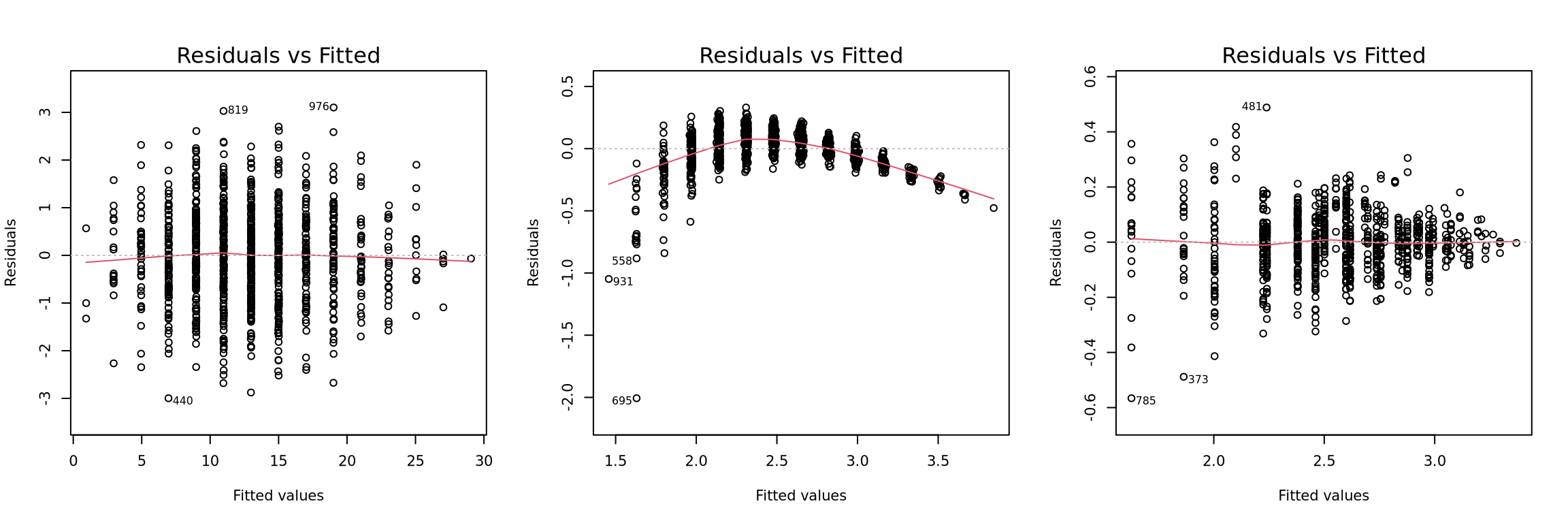
Figure 7.1: Three examples of Residual plot
A histogram of residuals can check the normality assumption. In the histogram, probability distribution of VMT is usually highly right-skewed. While the log-transformed VMT is more close to a bell curve. A better way is a normal quantile – quantile (QQ) plot of the residuals. An ideal cumulative normal distribution should plot as a straight line. Only looking at the \(R^2\) and p-values cannot disclose this feature.
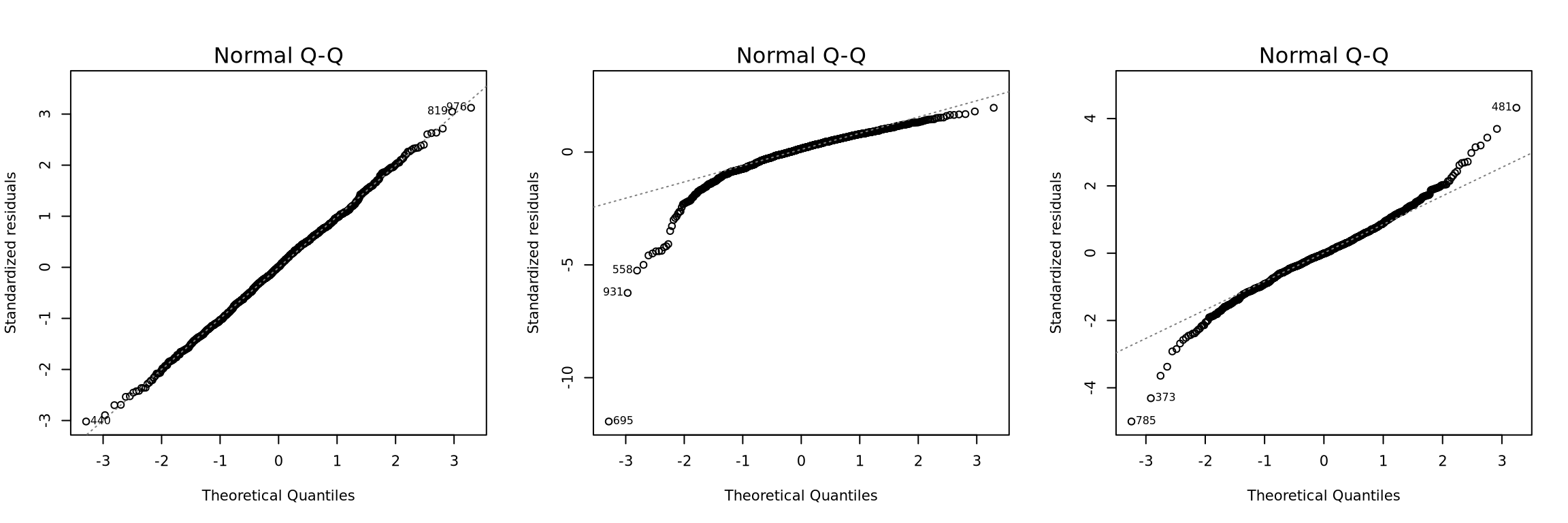
Figure 7.2: Three examples of Normal Q-Q Plot
- Goodness of fit
Coefficient of Determination \(R^2\) is a proportion to assess the quality of fitted model. This measurement tell us how good the model can explain the data.
\[\begin{equation} R^2 =\frac{SSR}{SST}=1-\frac{SSE}{SST} \tag{7.1} \end{equation}\]
when \(R^2\) is close to \(1\), the most of variation in response can be explained by the fitted model. Although \(R^2\) is not the only criteria of a good model, it is often available in most published papers. Recall the discussion in Part I, the aggregated data will eliminate the difference among individuals, households, or neighborhoods. In the new variance structure, \(SSE\) will be much less than disaggregated model. The \(R^2\) in many disaggregate studies are around 0.3, while the \(R^2\) in some aggregate studies can reach 0.8. A seriously underfitting model’s outputs could be biased and unstable.
A fact is that adding predictors into the model will never decrease \(R^2\). If a VMT-urban form model added many predictors but adjusted \(R^2\) is still low, the association between travel distance and built environment might be spurious. \(R^2\) also cannot reflect the different number of parameters in the models. Adjusted \(R^2\) can address this issue by introducing degree of freedom. The degree of freedom denotes the amount of information required to know.
\[\begin{equation} \begin{split} df_T =& df_R + df_E\\ n-1=&(p-1)+(n-p) \end{split} \tag{7.2} \end{equation}\]
Then, the mean square (MS) of each sum of squares (SS) can be calculated by \(MS=SS/df\). The mean square error \(MSE\) is also called as the expected value of error variance \(\hat\sigma^2=MSE=SSE/(n-p)\). \(n-p\) is the degree of freedom. Then adjusted \(R^2\) is
\[\begin{equation} R_{adj}^2 = 1-\frac{MSE}{MST} = 1-\frac{SSE/(n-p)}{SST/(n-1)} \tag{7.3} \end{equation}\]
Another similar method is \(R^2\) for prediction based on PRESS. Recall the PRESS statistic is the prediction error sum of square by fitting a model with \(n-1\) observations.
\[\begin{equation} PRESS = \sum_{i=1}^n(y_i-\hat y_{(i)})^2= \sum_{i=1}^n\left(\frac{e_i}{1-h_{ii}}\right)^2 \tag{7.4} \end{equation}\]
A model with smaller PRESS has a better ability of prediction. The \(R^2\) for prediction is
\[\begin{equation} R_{pred}^2 = 1-\frac{PRESS}{MST} \tag{7.5} \end{equation}\]
- Heterogeneity and Autocorrelation
For spatio-temporal data, the observations often have some relationship over time or space. When the assumption of constant variance is violated, the linear model has the issue of heterogeneity. When the assumption of independent errors is violated, the linear model with serially correlated errors is called autocorrelation. Spatial heterogeneity and spatial autocorrelation are two typical phenomenon in urban studies. All the neighboring geographic entities or stages could impact each other, or sharing the similar environment. Failing to deal with spatial heterogeneity could produce fake significance in hypothesis test and lead to systematically biased estimates. Although the estimation of coefficients could be unbiased when there is spatial autocorrelation in regression models, the estimated error variance would be biased and make misleading significance tests (Lianjun Zhang, Ma, and Guo 2009).
Here is a simple case of heterogeneous model. Recall Generalized least square estimates , if the residuals are independent but variances are not constant, a simple linear model becomes \(\boldsymbol{\varepsilon}\sim MVN(\mathbf{0},\sigma^2\mathbf{V})\) where \(\mathbf{V}\) is a diagonal matrix with \(v_{ii}=x^2_i\). Then \(\mathbf{X'V^{-1}X}=n\) and the weighted least squares solution is \(\hat\beta_{1,WLS}=\frac1n\sum_{i=1}^{n}\frac{y_i}{x_i}\) and \(\hat\sigma^2_{WLS}=\frac1{n-1}\sum_{i=1}^{n}\frac{(y_i-\hat\beta_{1}x_i)^2}{x_i^2}\). In this case, the OLS estimates of coefficients are still unbiased but no longer efficient. The estimates of variances are biased. The corresponding hypothesis test and confidence interval would be misleading.
If the data is aggregated to a upper level, it is the cases of geographic modifiable areal unit problem (MAUP) discussed in previous chapter. Let \(u_j\) and \(v_j\) are the response and predictors of \(j\)th household in a neighborhood. \(n_i\) is the sample size in each neighborhood. Then \(y_i=\sum_{j=1}^{n_i}u_j/n_i\) and \(X_i=\sum_{j=1}^{n_i}v_j/n_i\). Then \(\mathbf{X'V^{-1}X}=\sum_{i=1}^nn_ix_i^2\) and the WLS estimate of \(\beta_1\) is \(\hat\beta_{1,WLS}=\frac1n\frac{\sum_{i=1}^{n}n_ix_iy_i}{\sum_{i=1}^{n}n_ix_i^2}\) and \(V[\hat\beta_{1,WLS}]=\frac{\sigma^2}{\sum_{i=1}^{n}n_ix_i^2}\). There are three procedures, Bartlett’s likelihood ratio test, Goldfeld-Quandt test, or Breusch-Pagan test which can be used to examine heterogeneity (Ravishanker and Dey 2020, 8.1.3, pp.288–290)
Take a case of single dimension autocorrelation for example, it assumes the model have constant variance. That is \(E[\varepsilon]=0\). But \(Cov[\varepsilon_i,\varepsilon_j]=\sigma^2\rho^{|j-i|}\), \(i,j=1,2,...,n\) and \(|\rho|<1\) This is a linear regression with autoregressive order 1 (AR(1)). The estimates of \(\boldsymbol{\hat\beta}\) is the same with the GLS solutions, which are \(\boldsymbol{\hat\beta}_{GLS}=(\mathbf{X'V^{-1}X})^{-1}\mathbf{X'V^{-1}}\mathbf{y}\) and \(\widehat{V[\boldsymbol{\hat\beta}_{GLS}]}=\hat\sigma^2_{GLS}(\mathbf{X'V^{-1}X})^{-1}\), where \(\hat\sigma^2_{GLS}=\frac1{n-p}(\mathbf{y-X}\boldsymbol{\hat\beta}_{GLS})'\mathbf{V^{-1}}(\mathbf{y-X}\boldsymbol{\hat\beta}_{GLS})\). The variance-covariance matrix \(\mathbf{V}\) is also called Toeplitz matrix.
It is can be verified that \(\boldsymbol{\hat\beta}_{GLS}\le\boldsymbol{\hat\beta}_{OLS}\) always holds and they are equal when \(\mathbf{V=I}\) or \(\rho=0\). It proves that \(\boldsymbol{\hat\beta}_{GLS}\) are the best linear unbiased estimators (BLUE). This case can be extended to miltiple regression models and the autocorrelation of a stationary stochastic process at lag-k. Durbin-Watson test is used to test the null hypothesis of \(\rho=0\).
- A brief discussion
Only reporting the \(R^2\) and p-values cannot tell us whether the model is valid or not. Residual analysis can detect the ill-condition models and should not be ignored in regression studies.
For non-OLS model, such as logistic regression, \(R^2\) doesn’t exist. Pseudo \(R^2\)s are used to evaluate the goodness-of-fit. McFadden’s \(R^2\), Count \(R^2\), Efron’s \(R^2\) are some common Pseudo \(R^2\) with different interpretations. For example McFadden’s \(R^2\) use the ratio of the log likelihood to reflect how better is the full model than the null model. When examining the effects of built-environment factors on VMT at multiple spatial levels, Hong, Shen, and Zhang (2014) use a Bayesian version of adjusted \(R^2\) for multilevel models which proposed by Gelman and Pardoe (2006). Therefore, cross comparing \(R^2\) and various Pseudo \(R^2\) is meaningless. Pseudo \(R^2\)s on different data are also not comparable. Next question is what is a satisfactory model fit for different categories.
Some techniques can deal with spatial heterogeneity and autocorrelation and improve the model performance. More discussions of addressing spatial effects are placed on the next chapter.
7.3 Multicollinearity
Multicollinearity or near-linear dependence refers to the models with highly correlated predictors. When data is generated from experimental design, the treatments \(X\) could be fixed variables and be orthogonal. But travel-urban form model is observational studies and nothing can be controlled as in lab. It is known that there are complex correlations among the built-environment predictors themselves. Although, the basic IID assumptions do not require that all predictors \(\mathbf{X}\) are independent, when the predictors are near-linear dependent, the model is ill-conditioned and the least-square estimators are unstable.
- Variance Inflation
Multicollinearity can make the variances inflated and impact model precision seriously. If some of predictors are exact linear dependent, the matrix \((\mathbf{X'X})^{-1}\) is symmetric but non-invertible. By spectral decomposition of symmetric matrix, \(\mathbf{X'X}=\mathbf{P'\Lambda P}\) where \(\Lambda=\text{diag}(\lambda_1,...,\lambda_p)\), \(\lambda_i\)’s are eigenvalues of \(\mathbf{X'X}\), \(\mathbf{P}\) is an orthogonla matrix whose columns are normalize eigenvectors. Then the total-variance of \(\boldsymbol{\hat\beta}_{LS}\) is \(\sigma^2\sum_{j=1}^p1/\lambda_j\). If the predictors are near-linear dependent or nearly singular, \(\lambda_j\)s may be very small and the total-variance of \(\boldsymbol{\hat\beta}_{LS}\) is highly inflated. For the same reason, the correlation matrix using unit length scaling \(\mathbf{Z'Z}\) will has a inverse matrix with inflated variances. That means that the diagonal elements of \((\mathbf{Z'Z})^{-1}\) are not all equal to one. The diagonal elements are called Variance Inflation Factors, which can be used to examine multicollinearity. The VIF for a particular predictor is examined by \(\mathrm{VIF}_j=\frac{1}{1-R_j^2}\), where \(R_j^2\) is the coefficient of determination by regressing \(x_j\) on all the remaining predictors.
A common approach is to drop off the predictor with greatest VIF and refit the model until all VIFs are less than 10. However, dropping off one or more predictors will lose many information which might be valuable for explaining response. Due to the complexity among predictors, dropping off the predictor with the greatest VIF is not always the best choice. Sometimes, removing a predictor with moderate VIF can make all VIFs less than 10 in the refitted model. Moreover, there is not an unique criteria for VIF value. When the relationship between predictor and response is weak, or the \(R^2\) is low, the VIFs less than 10 may also affect the ability of estimation dramatically. Orthogonalization before fitting the model might be helpful. Other approaches such as principal components regression, ridge regression, etc. could deal with multicollinearity better.
- Principal Components Regression
Principal Components Regression (PCR) is a dimension reduction method which projecting the original predictors into a lower-dimension space. It still uses a singular value decomposition (SVD) and get \(\mathbf{X'X}=\mathbf{Q\Lambda Q}'\) \(\mathbf{Q}\) are the matrix who columns are orthogonal eigenvectors of \(\mathbf{X'X}\). \(\Lambda=\text{diag}(\lambda_1,...,\lambda_p)\) is decreasing eigenvalues with \(\lambda_1\ge\lambda_1\ge\cdots\ge\lambda_p\). Then the linear model can transfer to \(\mathbf{y} = \mathbf{XQQ}'\boldsymbol\beta + \varepsilon = \mathbf{Z}\boldsymbol\theta + \varepsilon\), where \(\mathbf{Z}=\mathbf{XQ}\), \(\boldsymbol\theta=\mathbf{Q}'\boldsymbol\beta\). \(\boldsymbol\theta\) is called the regression parameters of the principal components. \(\mathbf{Z}=\{\mathbf{z}_1,...,\mathbf{z}_p\}\) is known as the matrix of principal components of \(\mathbf{X'X}\). Then \(\mathbf{z}'_j\mathbf{z}_j=\lambda_j\) is the \(j\)th largest eigenvalue of \(\mathbf{X'X}\). PCR usually chooses several \(\mathbf{z}_j\)s with largest \(\lambda_j\)s and can eliminate multicollinearity. Its estimates \(\boldsymbol{\hat\beta}_{P}\) results in low bias but the mean squared error \(MSE(\boldsymbol{\hat\beta}_{P})\) is smaller than that of least square \(MSE(\boldsymbol{\hat\beta}_{LS})\).
- Ridge Regression
Least squares method gives the unbiased estimates of regression coefficients. However, multicollinearity will lead to inflated variance and make the estimates unstable and unreliable. To get a smaller variance, a tradeoff is to release the requirement of unbiasedness. Hoerl and Kennard (1970) proposed ridge regression to address the nonorthogonal problems. The estimates of ridge regression are \(\boldsymbol{\hat\beta}_{R}=(\mathbf{X'X}+k\mathbf{I})^{-1}\mathbf{X'}\mathbf{y}\), where \(k\ge0\) is a selected constant and is called a biasing parameter. When \(k=0\), the ridge estimator reduces to least squares estimators.
The advantage of ridge regression is to obtain a suitable set of parameter estimates rather than to improve the fitness. It could have a better prediction ability than least squares. It can also be useful for variable selection. The variables with unstable ridge trace or tending toward the value of zero can be removed from the model. In many case, the ridge trace is erratic divergence and may revert back to least square estimates. (Jensen and Ramirez 2010, 2012) proposed surrogate model to further improve ridge regression. Surrogate model chooses \(k\) depend on matrix \(\mathbf{X}\) and free to \(\mathbf{Y}\).
- Lasso Regression
Ridge regression can be understood as a restricted least squares problem. Denote the constraint \(s\), the solution of ridge coefficient estimates satisfies
\[\begin{equation} \min_{\boldsymbol\beta}\left\{\sum_{i=1}^n\left(y_i-\beta_0-\sum_{j=1}^p\beta_jx_j\right)^2\right\}\text{ subject to } \sum_{j=1}^p\beta_j^2\le s \end{equation}\]
Another approach is to replace the constraint term \(\sum_{j=1}^p\beta_j^2\le s\) with \(\sum_{j=1}^p|\beta_j|\le s\). This method is called lasso regression.
Suppose the case of two predictors, the quadratic loss function creates a spherical constraint for a geometric illustration, while the norm loss function is a diamond. The contours of \(\mathrm{SSE}\) are many expanding ellipses centered around least square estimate \(\hat\beta_{LS}\). Each ellipse represents a \(k\) value. If the restriction \(s\) also called ‘budget’ is very large, the restriction area will cover the point of \(\hat\beta_{LS}\). That means \(\hat\beta_{LS}=\hat\beta_{R}\) and \(k=0\). When \(s\) is small, the solution is to choose the ellipse contacting the constraint area with corresponding \(k\) and \(\mathrm{SSE}\). Here lasso constraint has sharp corners at each axes. When the ellipse has a intersect point on one corner, that means one of the coefficient equals zero. But it will not happen on ridge constraint. Therefore, an improvement of lasso with respect to ridge regression is that lasso allow some estimates \(\beta_j=0\). It makes the results more interpretative. Moreover, lasso regression can make variable selection.
- A brief discussion
Many studies such as Alam, Nixon, and Zhang (2018), check the multicollinearity issue after fitting the models. Using PCR method, some disaggregated travel models’ \(R^2\) can be over 0.5 (Hamidi and Ewing 2014; Tian et al. 2015). But the limitation is that the principal components are hard to interpret the meaning. The results of PCR may just describe the data themselves and they are reproducible but not replicable for other data.
Some research further investigate which variable plays the primary role. Using meta-regression, Gim (2013) find that accessibility to regional centers is the primary factor affecting travel behavior, while other D-variables are conditional or auxiliary factors.
Handy (2018) says most of the D-variable models have moderate multicollinearity issue and suggest to replace ‘Ds’ with ‘Accessibility’ framework. A question is, does the multicollinearity disappear in the new ‘A’ framework? Based on Handy (2005b) ’s suggestion, Proffitt et al. (2019) create an accessibility index by regression tree. It seems like multicollinearity is not the reason of choosing “D” or “A.”
To address multicollinearity, ridge regression, surrogate model, and lasso regression have provided plenty of choices. Tsao (2019) contribute another approach to handle multicollinearity which still uses ordinary least squares regression. Hence these ‘traditional’ methods are implementable and interpretative. More important is that they are comparable. Researcher maybe don’t need to rush into some more complex methods or post studies.
7.4 Variables Selections
For Multiple Linear Regression, variables selection is an essential step. But in travel-urban form literature this step often doesn’t take up much space. This section introduces several fundamental methods and discuss the related issues at the end.
- Selecting Procedure
Suppose the data has \(10\) candidate predictors. There will be \(1024\) possible models. All Possible Regressions fit all \(2^p\) models using \(p\) candidate predictors. Then one can select the best one based on above criteria. For high-dimension data, fitting all possible regressions is computing intensive and exhaust the degree of freedom. In practice, people often choose other more efficient procedures such as best-subset selection. Given a number of selected variables \(k\le p\), there could be \(p\choose k\) possible combinations. By fitting all \(p\choose k\) models with \(k\) predictors, denote the best model with smallest \(SSE\), or largest \(R^2\) as \(M_k\). For each \(k=1,2,...,p\), there will be \(M_0,M_1,...,M_p\) models. The final winner could be identified by comparing PRESS,
Stepwise selection include three methods: forward selection, backward elimination, and stepwise regression. Forward selection starts from null model with only intercept. In each step of this procedure, a variable with greatest simple correlation with the response will be added into the model. If the new variable \(x_1\) gets a large \(F\) statistic and shows a significance effect on response, the second step will calculate the partial correlations between two sets of residuals. One is from the new fitted model \(\hat y=\beta_0+\beta_1x_1\). Another one is the model of other candidates on \(x_1\), that is \(\hat x_j=\alpha_{0j}+\alpha_{1j}x_1\), \(j=2,3,...,(p-1)\). Then the variable with largest partial correlation with \(y\) is added into the model. The two steps will repeat until the partial \(F\) statistic is small at a given significant level. Backward elimination starts from the full model with all candidates. Given a preselected value of \(F_0\), each round will remove the variable with smallest \(F\) and refit the model with rest predictors. Then repeat to drop off one variable each round until all remaining predictors have a partial \(F_j>F_0\). Stepwise regression combines forward selection and backward elimination together. During the forward steps, if some added predictors have a partial \(F_j<F_0\), they also can be removed from the model by backward elimination. It is common that some candidate predictors are correlated. At the beginning, a predictor \(x_1\) having greater simple correlation with response was added into the model. However, along with a subset of related predictors were added, \(x_1\) could become ‘useless’ in the model. In this case, backward elimination is necessary for achieving the best solution.
Lasso regression can also help dropping off some variables. When reducing variance, lasso allow the least squares estimates shrinking towards zero. This method is called shrinkage.
- Model Evaluation Criteria
Coefficient of determination \(R^2\)is a basic measure of model performance. It has known that adding more predictor always increases \(R^2\). So the subset regression will stop to add new variables when the change of \(R^2\) is not significant. The improvement of \(R^2_{adj}\) is that it is not a monotone increasing function. So one can select a maximum value on a convex curve. Maximizing \(R^2_{adj}\) is equivalent to minimizing residual mean square \(\mathrm{MSE}\) When prediction of the mean response is the interest, \(R^2_{pred}\) based on prediction mean square error (PRESS) statistic is more preferred. PRESS is useful for selecting from two competing models.
Akaike Information Criterion (AIC) is a penalized measure using maximum entropy. AIC will decrease when adding extra terms into the model. Then one can justify when the model can stop adding the new terms. \(\mathrm{AIC}=n\ln\left(\frac1n \mathrm{SSE} \right)+ 2p\). Bayesian information criterion (BIC) is the extension of AIC. \(\mathrm{BIC}=n\ln\left(\frac{1}{n} \mathrm{SSE} \right)+ p\ln(n)\) Schwarz (1978) proposed a version of BIC with higher penalty for adding predictors when sample size is large.
Beside above criteria, Mallows \(C_p\) statistic is an important criteria related to the mean square error. Suppose the fitted subset model has \(p\) variables and expected response \(\hat y_i\). \(\mathrm{SSE}(p)\) is the total sum square error including two variance components. \(\mathrm{SSE}\) is the true sum square error from the ‘true’ model, while the sum square bias is \(\mathrm{SSE}_B(p)=\sum_{i=1}^n(E[y_i]-E[\hat y_i])^2= \mathrm{SSE}(p) - \mathrm{SSE}\). Then Mallows \(C_p=\frac{\mathrm{SSE}(p)}{\hat\sigma^2} - n + 2p\). If the supposed model is true, \(\mathrm{SSE}_B(p)=0\), it gives \(E[C_p|\mathrm{Bias}=0] = \frac{(n-p)\sigma^2}{\sigma^2}-(n-2p)=p\) Hence, a plot of \(C_p\) versus \(p\) can help to find the best one from many points. The proper model should have \(C_p\approx p\) and smaller \(C_p\) is preferred. \(C_p\) is often increase when \(\mathrm{SSE}(p)\) decrease by adding predictors. A personal judgment can choose the best tradeoff between smaller \(C_p\) and smaller \(\mathrm{SSE}(p)\).
- A brief discussion
The original data sources often include more than one hundred variables such as NHTS, ACS, LEHD, and EPA’s Smart Location Database. It is hard to conduct the systematic variable selections for all of them. In travel-urban form literature, the variables selections are mainly based on the background knowledge and research design. The framework conceived by D-variables allows researchers to add new candidates they favorite and compare the results. Aston et al. (2020) purpose that, in addition to D-variables, five explanatory variables are most common number in travel-urban form studies. Hence, for a target model with 10 covariates, above systematic methods of variables selection are still applicable.
For travel-urban form questions, researchers should also consider a target level of goodness-of-fit through variables selection. Due to data limitation or other reasons, one may only use a subset of the true predictors to fit the model, which is called underfitting. In social studies, underfitting is common because the social activities are very complex. Usual data collection could miss some important factors such as social network. Some psychological factors such as attitude or habit are hard to be quantified. Sometimes, the coefficients of determination are very low (e.g. \(R^2_{adj} = 0.0088\) (B. W. Lane 2011), \(R^2_{adj} = 0.085\) (Gordon et al. 2004, 27)).
In contrast, One may fit a model with extra irrelevant factors. Overfitting model fits the data too closely and may only capture the random noise. Or the extra factors are accidentally related to the response in this data. Some travel-urban form studies may have the risk of overfitting. For example, B. Lee and Lee (2013) ’s study applies two-stage least squares (2SLS) method and get \(R^2 = 0.96\). Sometimes high \(R^2\) may due to some specific research design or data source (e.g. \(R^2 = 0.979\) (J. Zhao et al. 2013), \(R^2 = 0.952\) (Cervero, Murakami, and Miller 2010)). Without suitable validation, many overfitting models produce false positive relationship and perform badly in prediction.