2.1 Probability functions for continuous random variables

For continuous random variables, the probability function is called a probability density function (PDF).

Example 2.1 (Probability density function) A rv $X$ has the uniform continuous distribution defined from $a$ to $b$ if the PDF is $f_X(x) = \left\{ \begin{array}{ll} \displaystyle \frac{1}{b-a} & \text{if $a<x<b$};\\[6pt] 0 & \text{otherwise}. \end{array} \right.$ This is usually written, for convenience, as $f_X(x) = \displaystyle \frac{1}{b-a}\quad \text{for $a<x<b$}.$

A PDF, say $f_X(x)$ (or just $f(x)$ when there is no ambiguity), has two properties:

$\displaystyle\int_{-\infty}^{\infty} f_X(x)\, dx = 1$ ; that is, the total probability is one (in other words, $x$ certainly must take some value).
$f_X(x) \ge 0$ for all $x$ ; that is, probabilities are non-negative.

Probabilities for continuous rvs are found by integrating over an appropriate area.

Example 2.2 (Uniform continuous distribution) A rv $X$ has the uniform continuous distribution defined from $50$ to $60$ if the PDF is $f_X(x) = \displaystyle \frac{1}{60-50} = \frac{1}{10} \quad\text{for $50<x<60$};$ see Fig. 2.1 (left panel). The probability that the $X$ takes a value between $50$ and $55$ is $\Pr(50<X<55) = \int_{50}^{55} f_X(x)\, dx = \int_{50}^{55} \frac{1}{10}\, dx = 0.5;$
see Fig. 2.1 (right panel). Note that the probability of observing any value exactly is zero since $X$ is continuous.

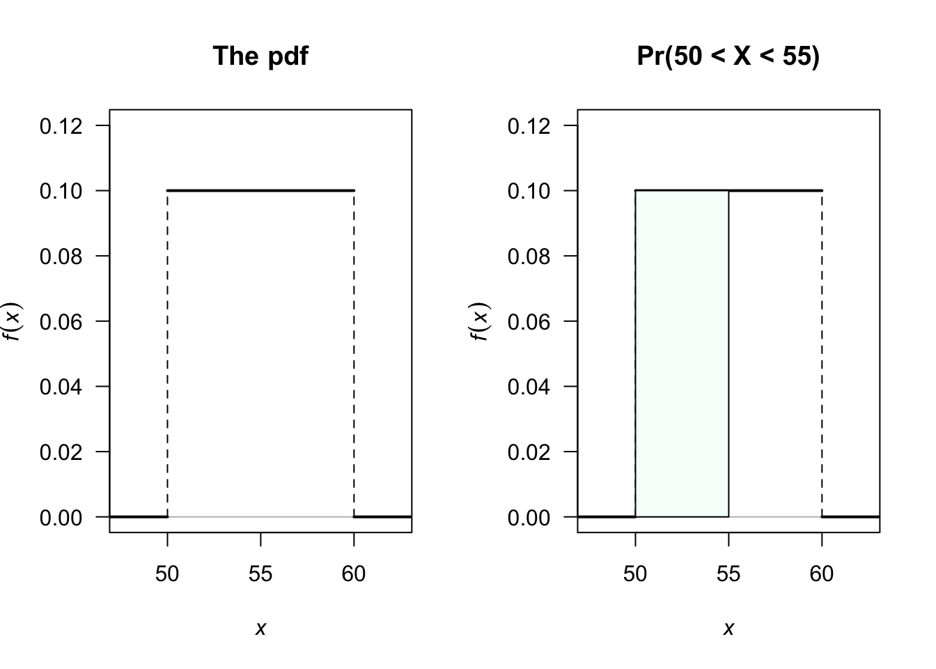
Left panel: A continuous uniform distribution defined for $50<x<60$. Right panel: Displaying the probability that the value of $X$ is between 50 and 55.

FIGURE 2.1: Left panel: A continuous uniform distribution defined for $50<x<60$ . Right panel: Displaying the probability that the value of $X$ is between 50 and 55.

Example 2.3 (PDF: Continuous rv) Consider a rv $Z$ with PDF $f_Z(z) = 3 z^2\quad\text{for $0<z<1$}.$ The probability that $z>0.5$ is $\Pr(Z>0.5) = 3 \int_{1/2}^{1} z^2 \, dz = z^3 \bigg\rvert_{z=1/2}^{z=1} = 1 - \frac{1}{8} = \frac{7}{8};$ see Fig.2.2.

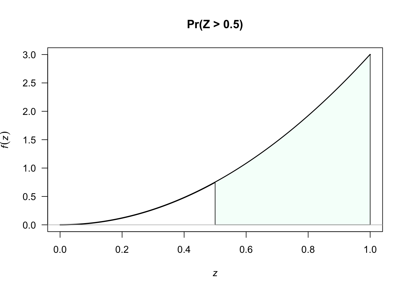
FIGURE 2.2: The PDF for the rv $Z$

Note that for $X$ continuous:

$\Pr(X=x) = 0$ for all values of $x$ .
Hence, $\Pr(a < X < b) = \Pr( a \le X < b) = \Pr(a < X \le b) = \Pr(a\le X\le b)$ .