2.4 Marginal distributions
A marginal distribution can be found by ‘integrating out’ (in the continuous case) the other variables. You can imagine looking at the joint probability function in (say) the \(x\)-direction, and accumulating the probability in that direction.
Example 2.8 (Rectangular sample space) For the joint probability distribution above, the marginal distribution for \(X\) is \[ f_X(x) = \int_{-1}^1 \frac{3(x + z^2)}{5}\, dz = \frac{2(3x+1)}{5} \] for \(0<x<1\). Note that this is a valid PDF.
Similarly, \[ f_Z(z) = \int_0^1 \frac{3(x + z^2)}{5}\, dx = \frac{3(1+2z^2)}{10} \] for \(-1 < z < 1\).
Example 2.9 (Non-rectangular sample space) Consider the PDF for two rvs \(X\) and \(Y\): \[ f_{X,Y}(x, y) = k (x+2y)\qquad\text{for $0<x<2$ and $0<y<(x/2)$}. \] To find the value of \(k\), we need to ensure the integral over the sample space \(S\) is one. Note that the sample space here is non-rectangular, so we need to be careful with the limits of integration; see Fig. 2.4. So proceed: \[\begin{align} 1 &=k\int_0^2\!\!\!\int_{y=0}^{y=x/2} (x+2y) \, dy\, dx\\ &= k \int_0^2 3x^2/4\, dx = 2k, \end{align}\] so we require that \(k=1/2\). The PDF is \(f_{X,Y}(x, y) = (x+2y)/2\) over the defined sample space.
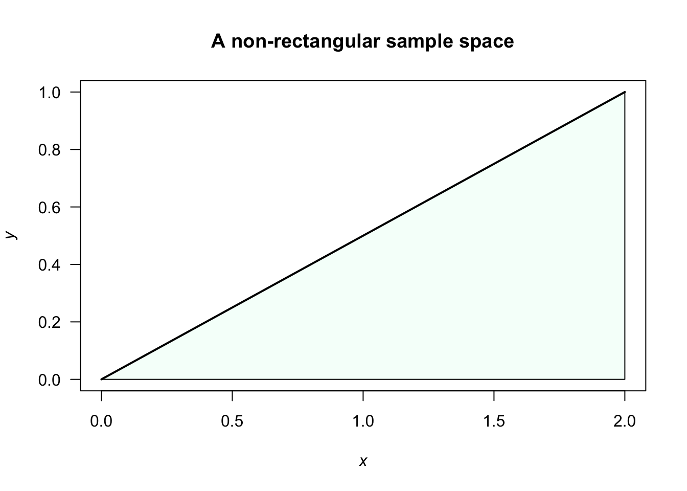
FIGURE 2.4: A non-rectangular sample space