7.2 Answers

1. Short answers:
   1. Since $x$ is defined over a continuous region, $X$ is a continuous rv.
   2. The cdf is found: $$F_Y(y) = \int_{-\infty}^x \lambda \exp(-\lambda t)\,dt = \Big| -\exp(-\lambda t)\Big|_{0}^x = -\exp(-\lambda x) + 1$$ since $\lambda > 0$. That is, the cdf is $F_Y(y) = 1 - \exp(-\lambda x)$ for $x > 0$, and $F_Y(y) = 0$ for $x \le 0$. See Fig. 7.1.
   3. There are two ways: $\int_3^\infty \exp(-x)\,dx$ (using the pdf), or $1 - F_Y(3)$ using the cdf. Either way, $\Pr(X > 3) = \exp(-3) \approx 0.0498$.
   4. By definition, $\displaystyle E[X] = \int_0^\infty x \lambda \exp(-\lambda x)\, dx$, which requires integration by parts; then $E[X] = 1/\lambda$.
      Also by definition, $\displaystyle E[X^2] = \int_0^\infty x^2 \lambda \exp(-\lambda x)\, dx$, which requires integration by parts twice; then $E[X] = 2/\lambda^2$. So $\text{var}[X] = E[X^2] - E[X]^2 = 1/\lambda^2$.

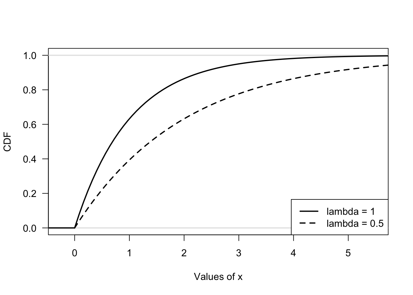
FIGURE 7.1: The CDF for Exercise 1

2. Short answers:
   1. Since $w$ is defined over a discrete region, $W$ is a discrete rv.
   2. To be a pmf, all probabilities must be non-negative (that is, $f_W(w) \ge 0$ for all $w$, which is true), and $\sum_S f_W(w) = 1$.
      For the second condition, use a result from the sum of a geometric series, that $\sum_0^\infty a r^k = a/(1 - r)$, where here $a = 0.6$ and $r = 0.4$.
   3. The cdf is: $$F_W(w) = \left\{ \begin{array}{ll} 0 & \text{for $W < 1$}\\ 0.6 & \text{for $1 \le W < 2$} \\ 0.6 + (0.6 \times 0.4) & \text{for $2 \le W < 3$}\\ 0.6 + (0.6 \times 0.4) + (0.6 \times 0.4^2) & \text{for $3 \le W < 4$}\\ \end{array} \right.$$ and a pattern can be seen to be developing. See Fig. 7.2.
   4. Here $\Pr(W > 2) = 1 - \Pr(W = 1) - Pr(W = 2)$, so $\Pr(W > 2) = 1 - 0.6 - (0.6\times 0.4) = 0.16$,
   5. You will need to use some results about sums of infinite series.

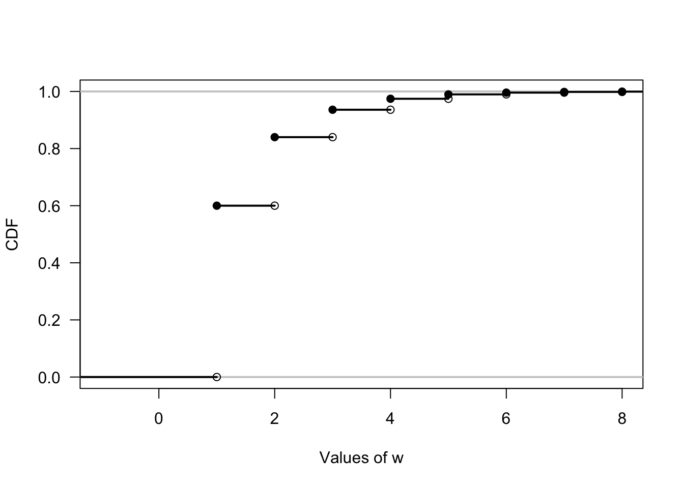
FIGURE 7.2: The CDF for Exercise 2

3. Short solutions (and see Exercise 1):
   1. We need $\int_W f_X(x)\, dx = 1$, so $\int_0^\infty k\exp(-x/4)\,dx = 1$. Solving, $k = 1/4$.
   2. The cdf is $F_X(x) = 1 - \exp(-x/4)$.
      See Fig. 7.3.
   3. $\Pr<X \le 2) = F_X(2) = 1 - \exp(-2/4) \approx 0.393$.
   4. $\Pr(2 < X < 4) = F_X(4) - F(X(2) \approx 0.239$.

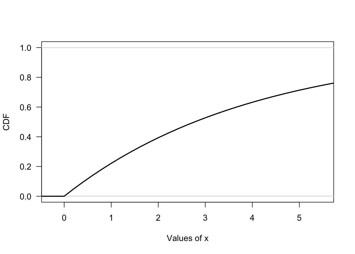
FIGURE 7.3: The CDF for Exercise 1

4. First we need to find the value of $k$, by solving $$1 = k \int_0^2 \!\!\! \int_0^1 3x^2 + xy\, dx\, dy,$$ showing that $k = 1/3$.
   Then the marginal distribution for $x$ is: $$f_X(x) = \frac{1}{3}\int_0^2 3x^2 + xy\, dy = 2x^2 + \frac{2x}{3}$$ for $0 < x < 1$.
   Also, the marginal distribution for $y$ is: $$f_Y(y) = \frac{1}{3}\int_0^1 3x^2 + xy\, dx = \frac{y + 2}{6}$$ for $0 < y < 2$.

5. This question has an irregular sample space, so care is needed!

   1. See Fig. 7.4.
   2. We need to solve $$1 = k \int_{z=0}^{z=1}\!\!\int_{y=0}^{y = z} y + z\, dy\, dz,$$ when we find that $k = 2$.

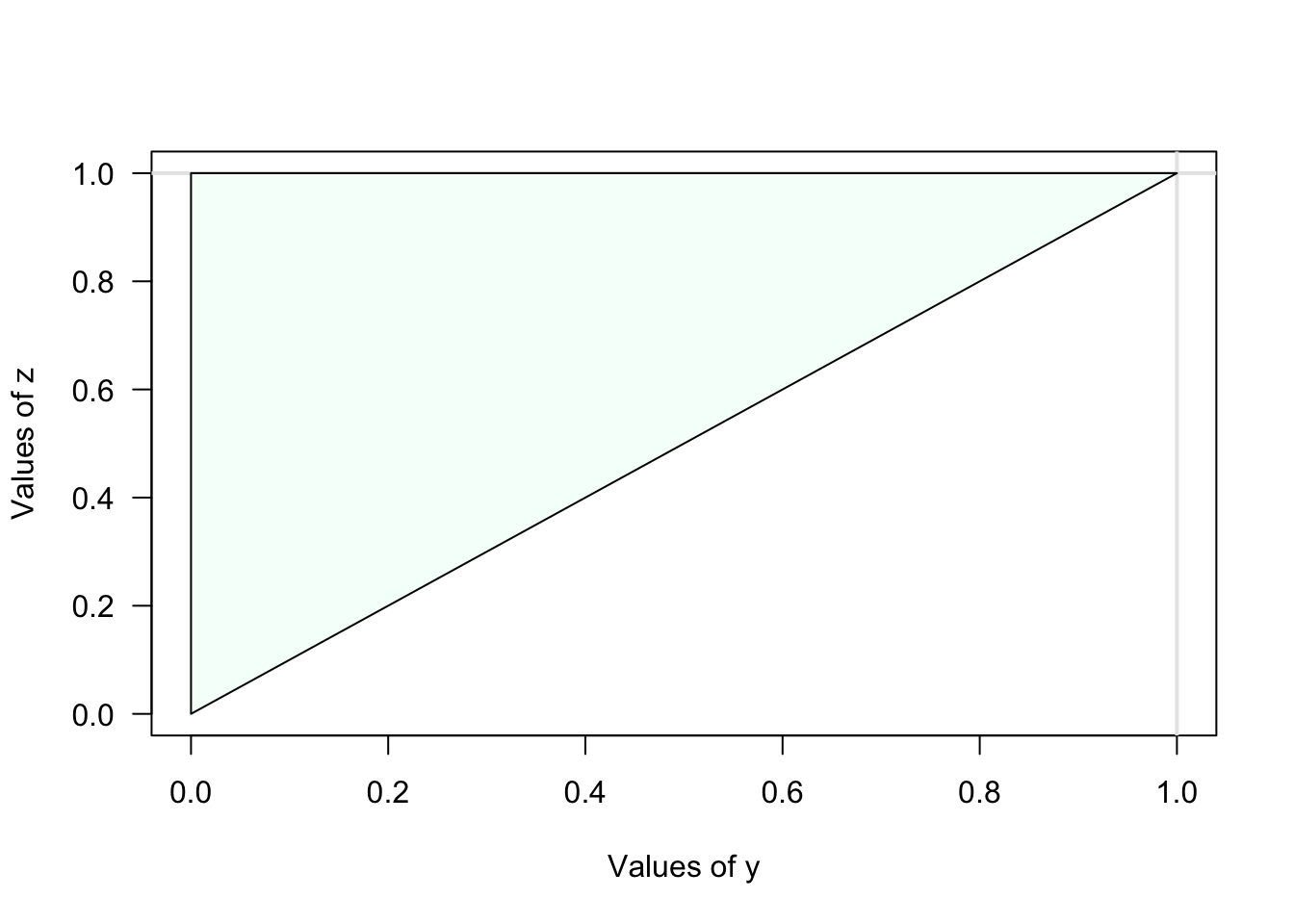
FIGURE 7.4: The sample space for Exercise 5

6. Proceed: $$\begin{align*} \text{Var}[ \bar{X} ] &= \text{Var}[ (X_1 + X_2 + \cdots + X_n)/n]\\ &= \frac{1}{n^2} \text{Var}[ X_1 + X_2 + \cdots + X_n ]\qquad \text{(since $\text{Var}[cX] = c^2\text{Var}[X]$))}\\ &= \frac{1}{n^2} \left( \text{Var}[ X_1] + \text{Var}[X_2] + \cdots + \text{Var}[X_n] \right)\\ &= \frac{1}{n^2} (n \times \sigma^2)\qquad \text{(since $\text{Var}(X) = \sigma^2$ for all $X$)}\\ &= \frac{\sigma^2}{n}. \end{align*}$$

---

Copyright © Peter K. Dunn, 2021