Listing 19.1: Compute Bayes Factor for Duck Game
(0.5^24 * 0.5^76) / (0.05^24 * 0.95^76)#> [1] 652.7191In Chapter 15, we learned how to turn a parameter estimation problem into a hypothesis test. In this chapter, we’re going to do the opposite: by looking at a virtually continuous range of possible hypotheses, we can use the Bayes factor and posterior odds (a hypothesis test) as a form of parameter estimation! This approach allows us to evaluate more than just two hypotheses and provides us with a simple framework for estimating any parameter.
N: 100, Success: 24 H1: p = 0.5 H2: p = 0.05
To get our Bayes factor, we need to compute P(D | H) for each hypothesis:
\[ \frac{P(D \mid H_{2}) = (0.05)^{24} \times (1 - 0.05)^{76}}{P(D \mid H_{1}) = (0.5)^{24} \times (1 - 0.5)^{76}} \tag{19.1}\]
Listing 19.1: Compute Bayes Factor for Duck Game
(0.5^24 * 0.5^76) / (0.05^24 * 0.95^76)#> [1] 652.7191Our Bayes factor tells us that \(H_{1}\), the attendant’s hypothesis, explains the data 653 times as well as \(H_{2}\).
This seems strange, because we got only 24 prices in 100 draws, which definitely is not near to 0.5.
Lets check with the pbinom() function (introduced in Chapter 13) to calculate the binomial distribution:
Listing 19.2: Compute probability of seeing 24 or fewer prizes, assuming that the probability of getting a prize is really 0.5
pbinom(24, 100, 0.5)#> [1] 9.050013e-08This is an extremely low value!
In the past, we’ve often found that the prior probability usually matters a lot when the Bayes factor alone doesn’t give us an answer that makes sense. … [But] there must be some problem here other than the prior.
One obvious problem is that, while it seems intuitively clear that the attendant is wrong in his hypothesis, the customer’s alternative hypothesis is just too extreme to be right, either, so we have two wrong hypotheses. What if the customer thought the probability of winning was 0.2, rather than 0.05? We’ll call this hypothesis \(H_{3}\). Testing \(H_{3}\) against the attendant’s hypothesis radically changes the results of our likelihood ratio:
\[ \frac{P(D \mid H_{3}) = (0.2)^{24} \times (1 - 0.2)^{76}}{P(D \mid H_{1}) = (0.5)^{24} \times (1 - 0.5)^{76}} \tag{19.2}\]
Listing 19.3: Compute Bayes Factor for Duck Game
(0.2^24 * 0.8^76) / (0.5^24 * 0.5^76)#> [1] 917399.4The trouble we had in our first hypothesis test was that the customer’s belief was a far worse description of the event than the attendant’s belief.
Of course, we haven’t really solved our problem. What if there’s an even better hypothesis out there?
We’ll consider every increment of 0.01 between 0 and 1 as a possible hypothesis.
Listing 19.4: Search with increment of 0.01 for als hypothesises between 0 and 1
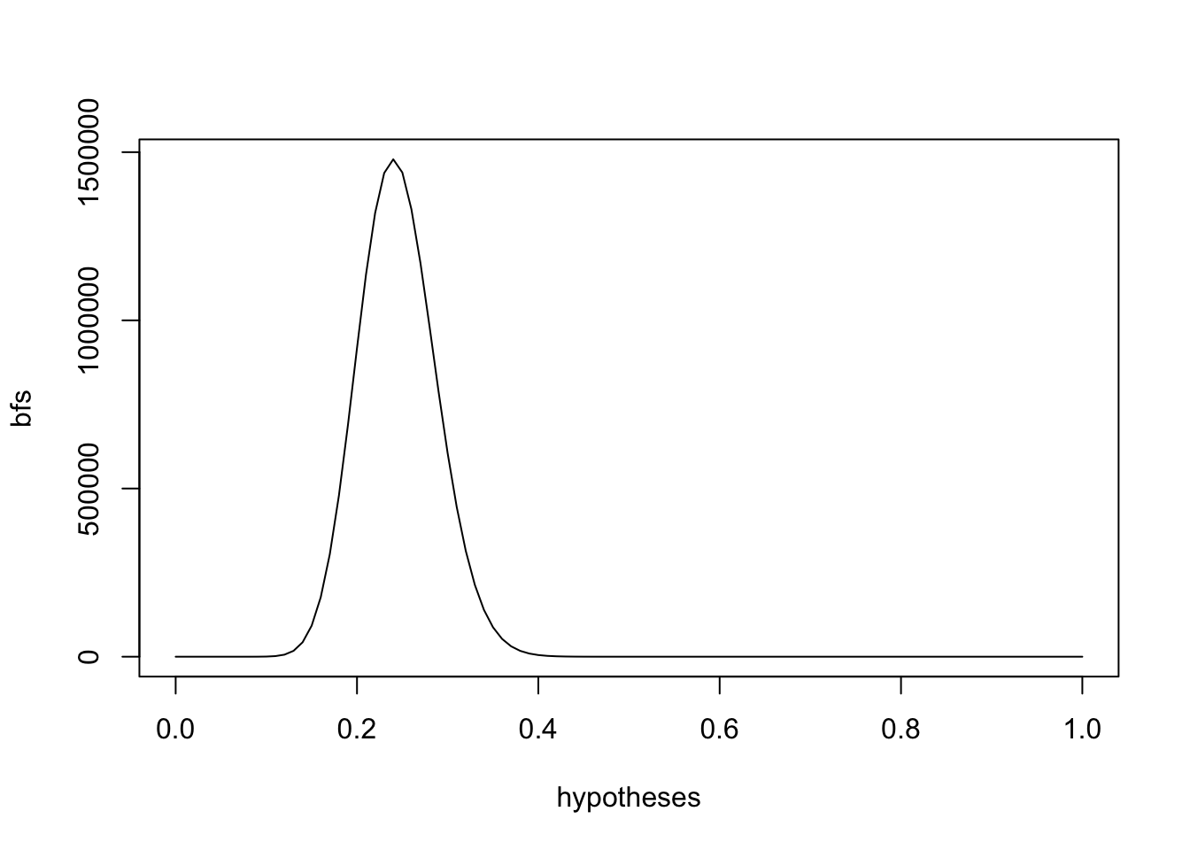
1.478776^{6} is the largest Bayes factor in our vector bfs. 0.24 is the highest likelihood ratio, telling us which hypothesis we should believe in the most.
I want to try this calculation with appropriate R packages. Maybe {BayesFactor} could be helpful?
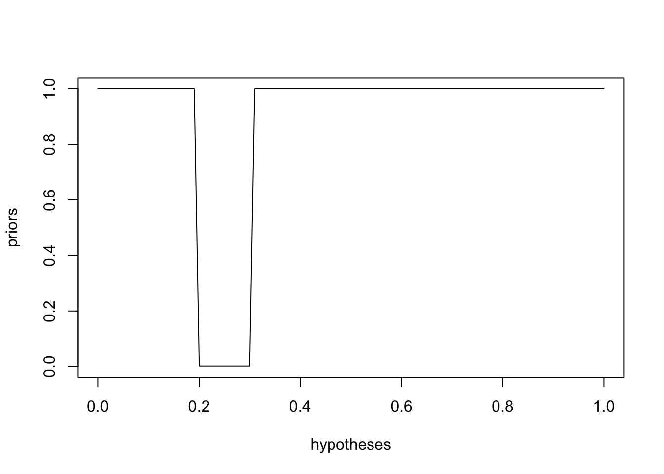
“I used to make games like these, and I can tell you that for some strange industry reason, the people who design these duck games never put the prize rate between 0.2 and 0.3. I’d bet you the odds are 1,000 to 1 that the real prize rate is not in this range. Other than that, I have no clue.”
Listing 19.5: Visualize the prior that the duck games never put a prize rate between 0.2 and 0.3
Listing 19.6: Plot new posterior distribution inlcuding the prior
posteriors <- priors * bfs
plot(hypotheses, posteriors, type = 'l')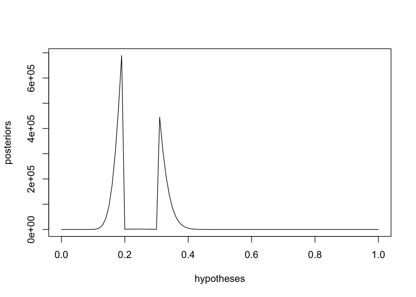
The posterior odds for our hypotheses is sum(posteriors) = 3.1406875^{6}, e.g. it does not sum to 1. So we need to normalize it by dividing each value in our posteriors vector by the sum of all the values: p.posteriors <- posteriors/sum(posteriors) = . Now sum(p.posteriors) adds to 1.
Listing 19.7: Plot the normalized posterior odds
plot(hypotheses, p.posteriors, type = 'l')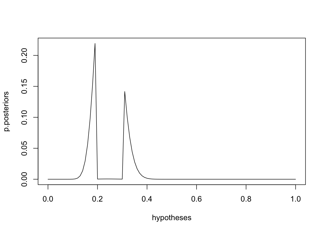
We can also use our p.posteriors to answer some common questions we might have about our data. For example, we can now calculate the probability that the true rate of getting a prize is less than what the attendant claims. We just add up all the probabilities for values less than 0.5:
sum(p.posteriors[which(hypotheses < 0.5)]) = 0.9999995
we can be almost certain that the attendant is overstating the true prize rate.
We can also calculate the expectation of our distribution and use this result as our estimate for the true probability. Recall that the expectation is just the sum of the estimates weighted by their value:
sum(p.posteriors * hypotheses) = 0.2402704
Of course, we can see our distribution is a bit atypical, with a big gap in the middle, so we might want to simply choose the most likely estimate, as follows:
hypotheses[which.max(p.posteriors)] = 0.19
Now we’ve used the Bayes factor to come up with a range of probabilistic estimates for the true possible rate of winning a prize in the duck game. This means that we’ve used the Bayes factor as a form of parameter estimation!
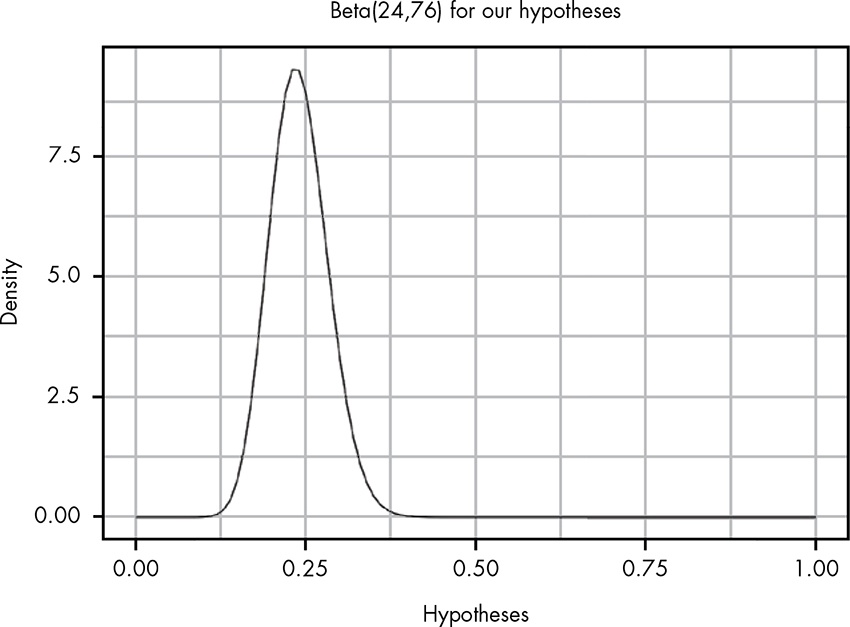
As we’ve discussed many times since Chapter 5, if we want to estimate the rate of some event, we can always use the beta distribution.
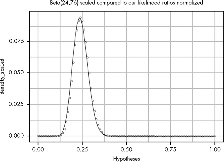
Except for the scale of the y-axis, the plot looks nearly identical to the original plot of our likelihood ratios! In fact, if we do a few simple tricks, we can get these two plots to line up perfectly. If we scale our beta distribution by the size of our
dxand normalize ourbfs, we can see that these two distributions get quite close:
There seems to be only a slight difference now. We can fix it by using the weakest prior that indicates that getting a prize and not getting a prize are equally likely—that is, by adding 1 to both the alpha and beta parameters
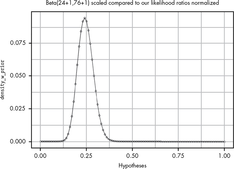
by using the Bayes factor, we’ve been able to empirically re-create a modified version of it that assumes a prior of Beta(1,1). And we did it without any fancy mathematics! All we had to do was:
- Define the probability of the evidence given a hypothesis.
- Consider all possible hypotheses.
- Normalize these values to create a probability distribution.
Not only is the Bayes factor a great tool for setting up hypothesis tests, but, as it turns out, it’s also all we need to create any probability distribution we might want to use to solve our problem, whether that’s hypothesis testing or parameter estimation. We just need to be able to define the basic comparison between two hypotheses, and we’re on our way.
From the basic rules of probability, we can derive Bayes’ theorem, which lets us convert evidence into a statement expressing the strength of our beliefs. From Bayes’ theorem, we can derive the Bayes factor, a tool for comparing how well two hypotheses explain the data we’ve observed. By iterating through possible hypotheses and normalizing the results, we can use the Bayes factor to create a parameter estimate for an unknown value. This, in turn, allows us to perform countless other hypothesis tests by comparing our estimates. And all we need to do to unlock all this power is use the basic rules of probability to define our likelihood, \(P(D \mid H)\)!
Try answering the following questions to see how well you understand using the Bayes factor and posterior odds to do parameter estimation. The solutions can be found at https://nostarch.com/learnbayes/.
Our Bayes factor assumed that we were looking at \(H_{1}: P(prize) = 0.5\). This allowed us to derive a version of the beta distribution with an alpha of 1 and a beta of 1. Would it matter if we chose a different probability for H1? Assume \(H_{1}: P(prize) = 0.24\), then see if the resulting distribution, once normalized to sum to 1, is any different than the original hypothesis.
Write a prior for the distribution in which each hypothesis is 1.05 times more likely than the previous hypothesis (assume our dx remains the same).
Suppose you observed another duck game that included 34 ducks with prizes and 66 ducks without prizes. How would you set up a test to answer “What is the probability that you have a better chance of winning a prize in this game than in the game we used in our example?” Implementing this requires a bit more sophistication than the R used in this book, but see if you can learn this on your own to kick off your adventures in more advanced Bayesian statistics!