8 The Prior, Likelihood, and Posterior of Bayes’ Theorem
8.1 The Three Parts
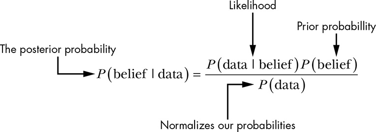
Bayes’ theorem has three parts:
- Prior Probability, \(P(belief)\)
- Likelihood, \(P(data | belief)\) and the
- Posterior Probability, \(P(belief | data)\).
The fourth part of Bayes’ theorem, probability of the data, \(P(data)\) is used to normalize the posterior so it accurately reflects a probability from 0 to 1. In practice, we don’t always need P(data), so this value doesn’t have a special name.
8.2 Investigating the Scene of a Crime
Kurt explains again Bayes’ theorem with an example: This time the probability of being robbed after finding that the is window broken, the front door is open, and a laptop is missing. One of the differences in the explanation with this example is the explicit use of the different parts of Bayes’ rule and the missing of data. He shows how to bypass missing data by comparing alternative hypotheses.
8.3 empty: Considering Alternative Hypotheses
8.4 Comparing Our Unnormalized Posteriors
If you compare alternative hypotheses than both the numerator and denominator contain P(data), so that you can remove it and still maintain the ratio.
8.5 empty: Wrapping Up
8.6 Exercises
Try answering the following questions to see if you have a solid understanding of the different parts of Bayes’ Theorem. The solutions can be found at https://nostarch.com/learnbayes/.
8.6.1 Exercise 8-1
As mentioned, you might disagree with the original probability \(P(robbed) = \frac{1}{1000}\) assigned to the likelihood:
\(P(\text{broken window, open front door, missing laptop | robbed}) = \frac{3}{10}\)
How much does this change our strength in believing \(H_{1}\) over \(H_{2}\)? (In the example in the text \(H_{1}\) explained what has observed 6,570 times better than \(H_{2}\). In the example the posterior probability of \(H_{2}\) was calculated with \(\frac{1}{21,900,000}\)
$$ \[\begin{align*} \frac{\frac{1}{1,000} \times \frac{3}{10}}{\frac{1}{21,900.000}} = \frac{\frac{3}{10,000}}{\frac{1}{21,900,000}} = \frac{65,700,000}{10,000} = 657 \end{align*}\] $$ The result still favors \(H_{1}\), but the difference is much smaller now.
8.6.2 Exercise 8-2
How unlikely would you have to believe being robbed is—our prior for \(H_{1}\)—in order for the ratio of \(H_{1}\) to \(H_{2}\) to be even?
$$ \[\begin{align*} \frac{\frac{1}{1,000} \times \frac{1}{21,900}}{\frac{1}{21,900.000}} = \frac{\frac{1}{21,900,000}}{\frac{1}{21,900,000}} = 1 \end{align*}\] $$ ::: {.callout-warning} I misunderstood the question of the exercise: I did not take into account the updated belief from Section 8.6.1. But the solution has the same principle: It would need an extremely unlikely belief, so that both hypotheses would be equally possible.
By the way: The high unlikeliness of \(H_{2}\) is a result in estimating each aspect of the data (broken window, open front door, and missing laptop) separately. Using the #eq-product-rule by multiplying the probability of all three events has resulted in an extremely low prior probability. I am therefore not sure if it is a good idea to estimate each factor individually. :::