Listing 4.1: Compute the binomial coefficient for flipping two heads in three tosses
choose(3,2)#> [1] 3A binomial distribution is used to calculate the probability of a certain number of successful outcomes, given a number of trials and the probability of the successful outcome. The “bi” in the term binomial refers to the two possible outcomes that we’re concerned with: an event happening and an event not happening. (If there are more than two outcomes, the distribution is called multinomial.)
Examples for a binomial distribution are:
Definition 4.1 (Parameter for the binomial distribution) All binomial distributions involve three parameters:
k The number of outcomes we care aboutn The total number of trialsp The probability of the event happeningCalculating the probability of flipping two heads in three coin tosses:
Theorem 4.1 (Shorthand notation of a binomial distribution) \[B(k; n, p) \tag{4.1}\]
For the example of two heads in three coin tosses, we would write \(B(2; 3, 1/2)\).
B stands for binomial distributionk is separated from the other parameters by a semicolon. This is because when we are talking about a distribution of values, we usually care about all values of \(k\) for a fixed \(n\) and \(p\).B(k; n, p) denotes each value in the distributionB(n, p) denotes the whole distributionWe’ll continue with the example of calculating the probability of flipping two heads in three coin tosses. Since the number of possible outcomes is small, we can quickly figure out the results we care about with just pencil and paper.
\[HHT, HTH, THH\] To start generalizing, we’ll break this problem down into smaller pieces we can solve right now, and reduce those pieces into manageable equations. As we build up the equations, we’ll put them together to create a generalized function for the binomial distribution.
Theorem 4.2 (Permuation Example for the Binomial Distribution)
\[ \begin{align*} P({heads, heads, tails}) = P({heads, tails, heads}) = P({tails, heads, heads}) = \\ P(\text{Desired Outcome}) \end{align*} \tag{4.2}\]
See how to do this calculation with R in Section 4.7.1.
There are three outcomes, but only one of them can possibly happen and we don’t care which. And because it’s only possible for one outcome to occur, we know that these are mutually exclusive, denoted as:
\[P(\{heads, heads, tails\},\{heads, tails, heads\},\{tails, heads, heads\}) = 0\] This makes using the sum rule of probability easy.
\[ \begin{align*} P(\{heads, heads, tails\} \operatorname{OR} \{heads, tails, heads\} \operatorname{OR} \{tails, heads, heads\}) = \\ P(\text{Desired Outcome}) + P(\text{Desired Outcome}) + P(\text{Desired Outcome}) = \\ 3 \times P(Desired Outcome) \end{align*} \] The value “3” is specific to this problem and therefore not generalizable. We can fix this by simply replacing “3” with a variable called \(N_{outcomes}\).
Theorem 4.3 (Solution with place holders) \[B(k;n,p) = N_{outcomes} \times P(\text{Desired Outcome}) \tag{4.3}\]
Now we have to figure out two subproblems:
First we need to figure out how many outcomes there are for a given k (the outcomes we care about) and n (the number of trials). For small numbers we can simply count. But it doesn’t take much for this to become too difficult to do by hand. The solution is combinatorics.
There is a special operation in combinatorics, called the binomial coefficient, that represents counting the number of ways we can select k from n — that is, selecting the outcomes we care about from the total number of trials.
Theorem 4.4 (Notation for the binomial coefficient) \[\binom{n}{k} \tag{4.4}\]
We read this as “n choose k”. In our example we would say “in three tosses choose two heads”:
\[\binom{3}{2}\]
Theorem 4.5 (Definition of the binomial coefficient operation) \[\binom{n}{k} = \frac{n!}{k! \times (n-k)!} \tag{4.5}\]
The ! means factorial, which is the product of all the numbers up to and including the number before the ! symbol, so \(5! = (5 × 4 × 3 × 2 × 1)\).
In R we compute the binomial coefficient for the case of flipping two heads in three tosses with the following function call:
Listing 4.1: Compute the binomial coefficient for flipping two heads in three tosses
choose(3,2)#> [1] 3See how to calculate the binomial coefficient with Base R in Section 4.7.2.
We can now replace \(N_{Outcomes}\) in Equation 4.3 with the binomial coefficient:
\[B(k;n,p) = \binom{n}{k} \times P(\text{Desired Outcome})\]
All we have left to figure out is the \(P(\text{Desired Outcome})\), which is the probability of any of the possible events we care about. So far we’ve been using \(P(\text{Desired Outcome})\) as a variable to help organize our solution to this problem, but now we need to figure out exactly how to calculate this value.
Let’s focus on a single case of our example of tow heads in three tosses: \(HHT\). Using the product rule and negation from the previous chapter, we can describe this problem as: \[P(heads, heads, no heads) = P(heads, heads, 1-heads)\] Now we can use the product rule from Equation 3.1:
\[
\begin{align*}
P(heads, heads, 1-heads) = \\
P(heads) \times P(heads) \times (1-P(heads)) = \\
P(heads)^2 \times (1-P(heads))^1
\end{align*}
\] You can see that the exponents for \(P(heads)^2\) and \(1 – P(heads)^1\) are just the number of heads and the number of not heads in our scenario. These equate to k, the number of outcomes we care about, and n – k, the number of trials minus the outcomes we care about. Puting all together:
\[
\binom{n}{k} \times P(heads)^{k} \times (1- P(heads))^{n-k}
\] Generalizing for any probability, not just heads, we replace \(P(heads)\) with just p. This gives us a general solution. Compare the following list with Definition 4.1.
k, the number of outcomes we care about;n, the number of trials; andp, the probability of the individual outcome.Theorem 4.6 (Probability Mass Function (PMF) for the Binomial Distribution) \[ \binom{n}{k} \times p^{k} \times (1- p)^{n-k} \tag{4.6}\]
Equation 4.6 is the basis of the binomial distribution. It is called a Probability Mass Function (PMF). The mass part of the name comes from the fact that we can use it to calculate the amount of probability for any given k using a fixed n and p, so this is the mass of our probability.
Now that we have this equation, we can solve any problem related to outcomes of a coin toss. For example, we could calculate the probability of flipping exactly 12 heads in 24 coin tosses:
\[ B(12,24,\frac{1}{2}) = \binom{24}{12} \times (\frac{1}{2})^{12} \times (1-\frac{1}{2})^{24-12} = 0.1611803 \]
Listing 4.2: Calculate the probability of flipping exactly 12 heads in 24 coin tosses
choose(24,12) * (1 / 2)^(12) * (1 - 1/2)^(24 - 12)#> [1] 0.1611803The calculation in Listing 4.2 is only valid for our concrete example.
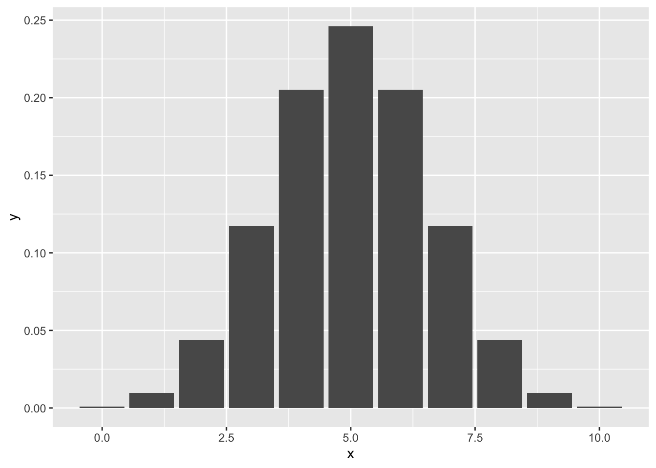
For example, we can plug in all the possible values for k in 10 coin tosses into our PMF and visualize what the binomial distribution looks like for all possible values.
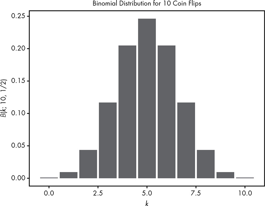
See my Figure 4.4 as a replication of Figure 4.1.
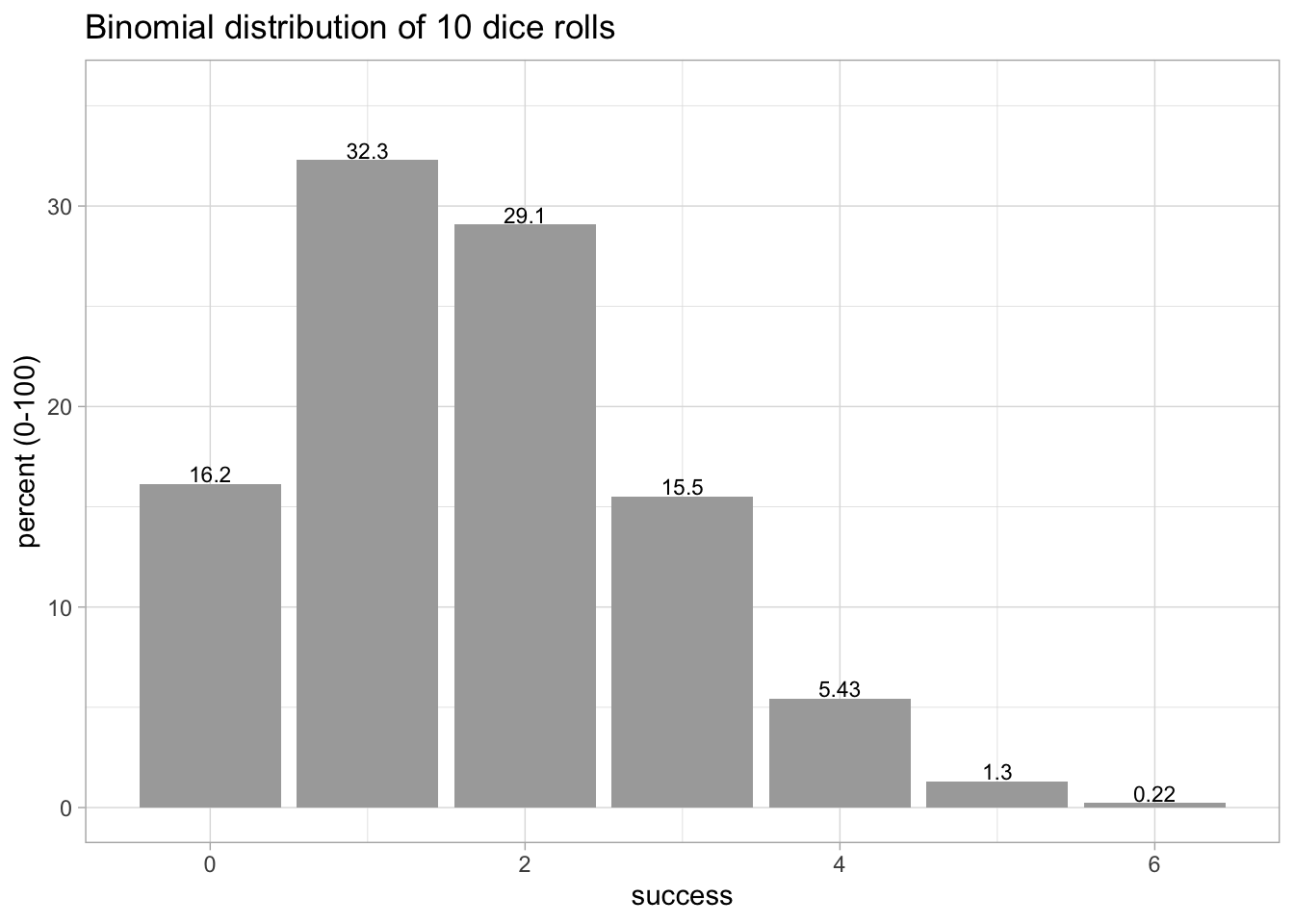
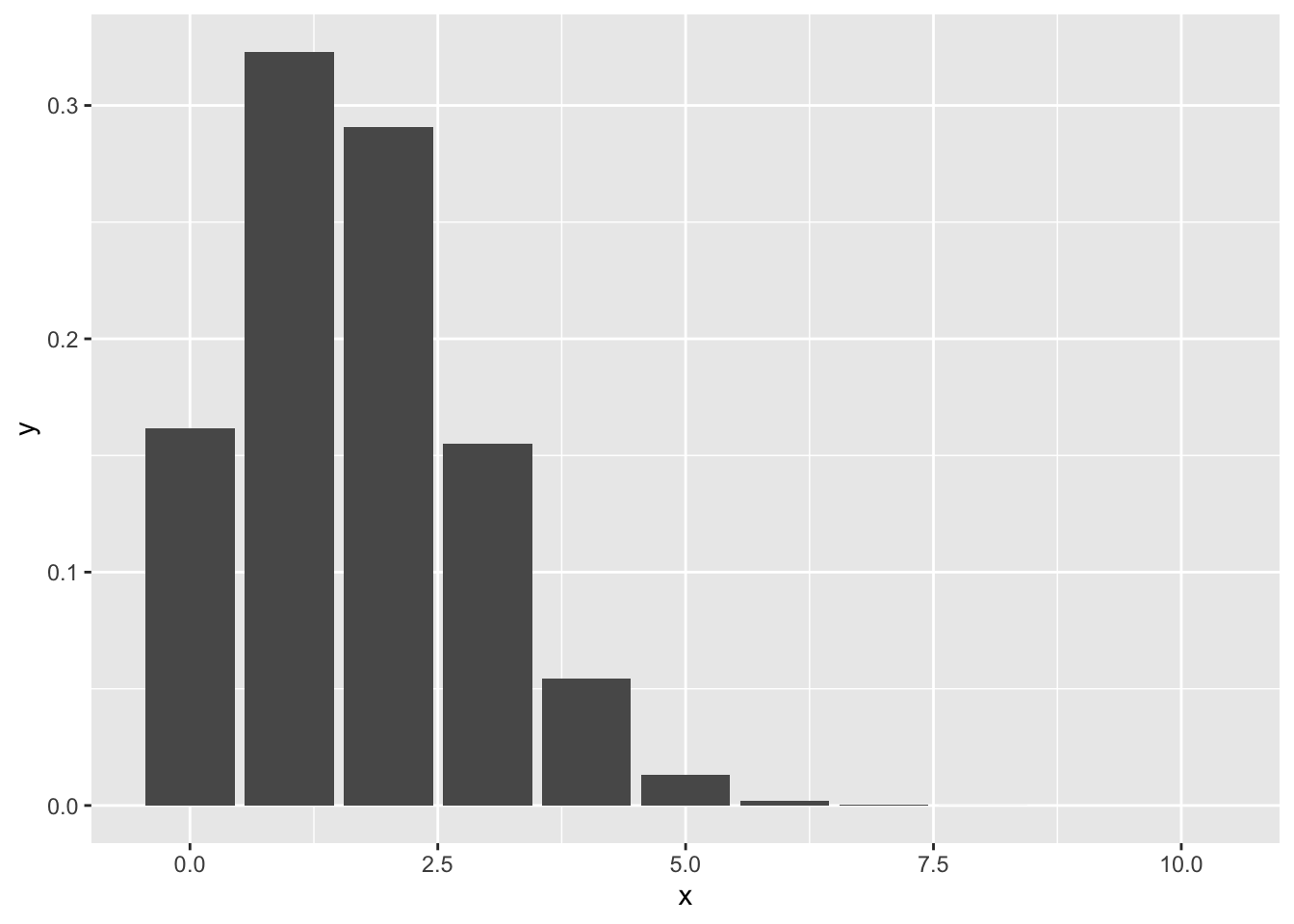
We can also look at the same distribution for the probability of getting a 6 when rolling a six-sided die 10 times, as shown in Figure 4.2.
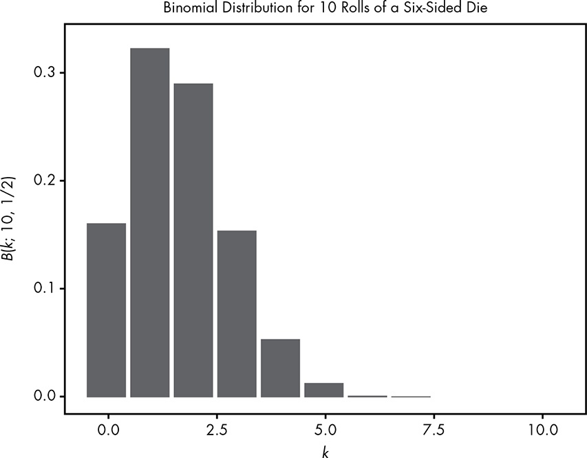
Again I replicated Figure 4.2 with my Figure 4.6.
Bottom line of the discussion in this section: A probability distribution is a way of generalizing an entire class of problems.
There is only one new content in this section: Instead of computing the probability of one event we are going to calculate the possibility of drawing at least one specific card from a pile of infinite numbers of cards where we know the probability of this card we are interested. The aim is to have a p of at last 50% with 100 trials and a probability of 0.720% for the card we are interested.
At first let us compute the probability for getting exactly one card we are interested with 100 draws form the pile. We know the probability to draw the featured card is 0.720%.
\[\binom{100}{1} \times 0.00720^{1} \times (1- 0.00720)^{100-1}\]
Listing 4.3: Draw exact one card that has p = 0.720%
dbinom(1, 100, 0.00720)#> [1] 0.352085And now let’s compute the probability for at least one card we are interested.
In R, we can use the Binomial Cumulative Distribution Function pbinom() to automatically sum up all the values of the card we are interested in our PMF.
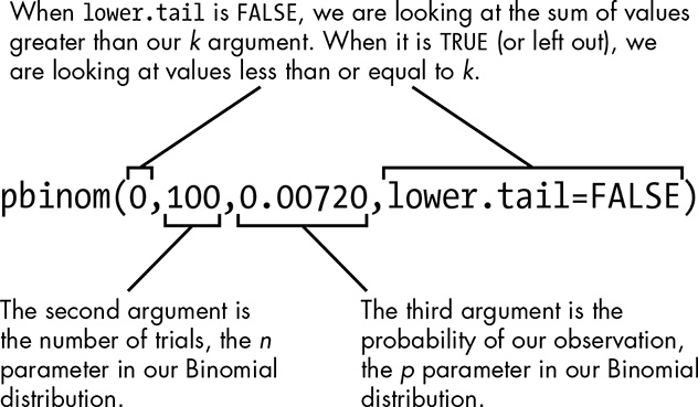
The pbinom() function takes three required arguments and an optional fourth called lower.tail (which defaults to TRUE). When the fourth argument is TRUE, the first argument sums up all of the probabilities less than or equal to our argument. When lower.tail is set to FALSE, it sums up the probabilities strictly greater than the first argument. By setting the first argument to \(0\), we are looking at the probability of getting one or more the cards we are interested. We set lower.tail to FALSE because that means we want values greater than the first argument (by default, we get values less than the first argument).
Listing 4.4: Example Calculation with the pbinom() Function
pbinom(0, 100, 0.00720, lower.tail = FALSE)#> [1] 0.5145138Voilá! This is the same result as in @#fig-pbinom-function.
In this chapter Will Kurt demonstrated how we can deduce intuitively the formula for the binomial coefficient.
I have seen this monstrosity of expression for the binomial coefficient many times in different books and was always overwhelmed from its complexity. But this has changed now: Will Kurt succeeded to demystify the formula for me!
Try answering the following questions to make sure you’ve grasped binomial distributions fully. The solutions can be found at https://nostarch.com/learnbayes/.
Exercise 4.1 What are the parameters of the binomial distribution for the probability of rolling either a 1 or a 20 on a 20-sided die, if we roll the die 12 times?
Listing 4.5: Binomial distribution for the probability of rolling either a 1 or a 20 on a 20-sided die, if we roll the die 12 times
dbinom(2, 12, 2/20)#> [1] 0.2301278Exercise 4.2 There are four aces in a deck of 52 cards. If you pull a card, return the card, then reshuffle and pull a card again, how many ways can you pull just one ace in five pulls?
Listing 4.6: If you pull a card, return the card, then reshuffle and pull a card again, how many ways can you pull just one ace in five pulls?
combinat::combn(x = 1:5, m = 1, fun = tabulate, simplify = TRUE, nbins = 5)#> [,1] [,2] [,3] [,4] [,5]
#> [1,] 1 0 0 0 0
#> [2,] 0 1 0 0 0
#> [3,] 0 0 1 0 0
#> [4,] 0 0 0 1 0
#> [5,] 0 0 0 0 1Listing 4.7: If you pull a card, return the card, then reshuffle and pull a card again, how many ways can you pull just one ace in five pulls?
choose(5,1)#> [1] 5In contrast to the result in the solution manual I programmed the exercise with combinat::combn(). This correct solution pretends that I could use it for every possible arrangement. That is not true. For instance I could not manage to display the many ways of rolling two 6s in three rolls of a six-sided die.
Exercise 4.3 For the example in Exercise 4.2, what is the probability of pulling five aces in 10 pulls (remember the card is shuffled back in the deck when it is pulled)?
Listing 4.8: Probability of pulling five aces in 10 pulls with replacing
dbinom(5, 10, 4 / 52) * 100#> [1] 0.04548553Only about 0.0455%. But this is different than the result in the solution manual with 1/32000 = 0.003125%. I don’t know why there is this difference.
Exercise 4.4 When you’re searching for a new job, it’s always helpful to have more than one offer on the table so you can use it in negotiations. If you have a 1/5 probability of receiving a job offer when you interview, and you interview with seven companies in a month, what is the probability you’ll have at least two competing offers by the end of that month?
Listing 4.9: Probability of at least 2 interviews each with 1/5 chance for a job offer having 7 interviews
pbinom(1, 7, 1/5, lower.tail = FALSE)#> [1] 0.4232832There is chance of about 42% that you receive at least two job offers.
In my first trial I calculated wrongly the probability for exact 2 competing offers with dbinom(2, 7, 1/2) instead of at least 2 competing offers! Additionally I forgot to add lower.tail = FALSE. to calculate more than x: x = 1, more than 1 = 2, therefore the first parameter is 1 (and not 2 as could be thought wrongly). Not using lower.tail = FALSE means that the default value of lower.tail = TRUE computes the probability of \(P[X <= x]\) (instead of \(P[X > x]\)).
Exercise 4.5 You get a bunch of recruiter emails and find out you have 25 interviews lined up in the next month. Unfortunately, you know this will leave you exhausted, and the probability of getting an offer will drop to 1/10 if you’re tired. You really don’t want to go on this many interviews unless you are at least twice as likely to get at least two competing offers. Are you more likely to get at least two offers if you go for 25 interviews, or stick to just 7?
Listing 4.10: Probability of at least 2 interviews each with 1/10 chance for a job offer having 25 interviews
pbinom(1, 25, 1/10, lower.tail = FALSE)#> [1] 0.7287941With a reduced probability per interview you raised your changes from 42,3% to 72,9%. But to get an job offer is not twice as likely so you stick with 7 interviews.
I want to get the same result as in Equation 4.2, but this time using R. What are the permutations of possible events by flipping two heads in three coin tosses?
Let’s P(heads) = 1 and P(tails) = 0, then we can use combinat::combn(). The package {combinat} is not part of Base R, so you have to install it.
Listing 4.11: Permutations of possible events by flipping two heads in three coin tosses
#>      [,1] [,2] [,3]
#> [1,]    1    1    0
#> [2,]    1    0    1
#> [3,]    0    1    1
The syntax is: combn(x, m, fun = NULL, simplify = TRUE, ...).
x: vector source for combinations equivalent to the the number of events.m: number of elements we are interested infun = function to be applied to each combination (may be null). I am using the base::tabulate() to take the integer-valued vector and counting the number of times each integer occurs in it.simplify: logical, if FALSE, returns a list, otherwise returns vector or array....: arguments for the used function. In our case nbins refers to the number of bin used by the tabulate() function.Let’s try another example to understand better the pattern of the combn() functions: What are the permutations of possible events by flipping a coin 5 times and getting three heads:
Listing 4.12: Permutations of possible events by flipping two heads in five coin tosses
combinat::combn(x = 1:5, m = 2, fun = tabulate, simplify = TRUE, nbins = 5)#> [,1] [,2] [,3] [,4] [,5] [,6] [,7] [,8] [,9] [,10]
#> [1,] 1 1 1 1 0 0 0 0 0 0
#> [2,] 1 0 0 0 1 1 1 0 0 0
#> [3,] 0 1 0 0 1 0 0 1 1 0
#> [4,] 0 0 1 0 0 1 0 1 0 1
#> [5,] 0 0 0 1 0 0 1 0 1 1There is also a special package {dice} for the calculation of various dice-rolling events. We could for instance compute the probability “What is the probability of rolling two 6s in three rolls of a six-sided die?” directly with:
Listing 4.13: Compute the probability of rolling two 6s in three rolls of a six-sided die
dice::getEventProb(nrolls = 3,
                   ndicePerRoll = 2,
                   nsidesPerDie = 6,
                   eventList = list(6, 6))
#> [1] 0.052512Actually I did not understand the many implications of computing combinations and / or permutations with different functions and different packages:
utils::combn()combinat::combn()gtools::combinations() and gtools::permutations()
permute::permute(), permute::shuffle()
base::expand.grid()tidyr::expand(), tidyr::crossing(), tidyr::nesting(), tidyr::expand_grid()
As far as I understand from my study of the Statistical Rethinking book, these functions are an important topic to understand Bayesian Statistics. These types of functions are used for grid approximation and in Bayesian statistics to extract or draw samples from fit models (e.g., rethinking::extract.samples(), rethinking::extract.prior())
I am sure I will need to come back to this issue and study available material more in detail! But at the moment I am stuck and will skip this subject.
I want to replicate the Base R function chosse() with Equation 4.5. This involves to calculate factorials with the base::factorial() function.
\[\binom{n}{k} = \frac{n!}{k! \times (n-k)!}\]
Listing 4.14: Calculate the probability of flipping exactly 12 heads in 24 coin tosses
#> [1] TRUECalculation of \(\binom{24}{12}\):
choose(24, 12) = 2.704156^{6}.my_choose(24, 12) = 2.704156^{6}.To generalize I write my own function for the density of the binomial distribution. I will use the same arguments names as in Definition 4.1.
Listing 4.15: Function for the density of the binomial distribution
my_dbinom <- function(k, n, p) {
    choose(n, k) * p^k * (1 - p)^(n - k)
}

my_dbinom(12, 24, 0.5)
#> [1] 0.1611803Voilá: It gives the same result as the manual calculation in Listing 4.2.
I wonder if there is not a Base R function which does the same as my_dbinom(). I tried stats::dbinom() and it worked!
Listing 4.16: Base R dbinom() function calculates the density of the binomial distribution
dbinom(12, 24, 0.5)#> [1] 0.1611803Again the same result as in Listing 4.2 and Listing 4.15!
Here I am going to try to replicate Figure 4.1.
Listing 4.17: Replicate Figure 4.1: Binomial Distribution of 10 Coin Flips
Writing Listing 4.17 I had troubles applying the correct geom. At first I used geom_bar() but this did not work until I learned that I have to add the option “stat = identity” or to use geom_col(). The difference is:
geom_bar() makes the height of the bar proportional to the number of cases in each group. It uses stat_count() by default, e.g. it counts the number of cases at each x position. If there aren’t cases but only the values then one has to add “stat = identity” to declare that ggplot2 should take the data “as-is”.geom_col() instead takes the heights of the bars to represent values in the data. It uses stat_identity() and leaves the data “as-is” by default.During my research for writing Listing 4.17 I learned of the {tidydice} package. It simulates dice rolls and coin flips and can be used for teaching basic experiments in introductory statistics courses.
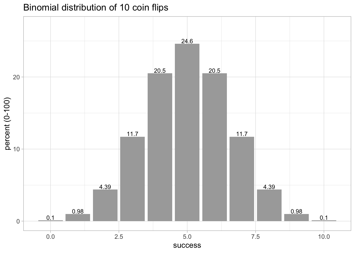
With {tidydice} we replicate Figure 4.1 with just 2 lines using the binom_coin() inside the plot_binom() function. In addition to the graphical distribution it print also the exact values on top of the bars.
Listing 4.18: Replicate Figure 4.1: Binomial Distribution of 10 Coin Flips {tidydice}
tidydice::plot_binom(
  tidydice::binom_coin(times = 10, sides = 2, success = 2),
  title = "Binomial distribution of 10 coin flips"
)
{tidydice} has many other functions related to coin and dice experiments.
I will replicate Figure 4.2 with {ggplot2} and with {tidydice}:
Listing 4.19: Replicate Figure 4.2: Binomial Distribution of 10 Dice Rolls
Listing 4.20: Replicate Figure 4.2: Binomial Distribution of 10 Dice Rolls {tidydice}
tidydice::plot_binom(
  tidydice::binom_dice(times = 10, sides = 6, success = 6),
  title = "Binomial distribution of 10 dice rolls"
)