13Tools of Parameter Estimation: The PDF, CDF, and Quantile Function
This chapter will cover more on the probability density function (PDF); introduce the cumulative distribution function (CDF), which helps us more easily determine the probability of ranges of values; and introduce quantiles, which divide our probability distributions into parts with equal probabilities. For example, a percentile is a 100-quantile, meaning it divides the probability distribution into 100 equal pieces. (115)
13.1 Estimating the Conversion Rate for an Email Signup List
Say you run a blog and want to know the probability that a visitor to your blog will subscribe to your email list. In marketing terms, getting a user to perform a desired event is referred to as the conversion event, or simply a conversion, and the probability that a user will subscribe is the conversion rate.
As discussed in Section 5.2, we would use the beta distribution to estimate p, the probability of subscribing, when we know k, the number of people subscribed, and n, the total number of visitors. The two parameters needed for the beta distribution are α, which in this case represents the total subscribed (k), and β, representing the total not subscribed (n – k).
13.2 The Probability Density Function
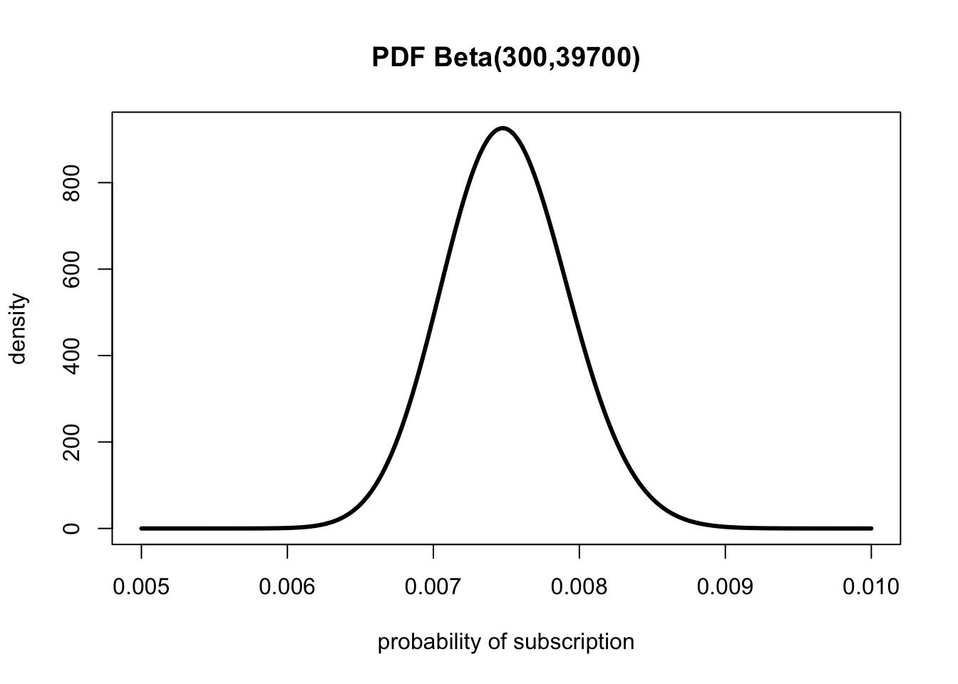
let’s say for the first 40,000 visitors, you get 300 subscribers. The PDF for our problem is the beta distribution where α = 300 and β = 39,700.
Theorem 13.1 (Computing the mean of the beta distribution) \[
\begin{align*}
\mu_{Beta} = \frac{\alpha}{\alpha + \beta} \\
\mu_{Beta} = \frac{300}{300 + 39,700} = 0.0075
\end{align*}
\tag{13.1}\]
The blog’s average conversion rate is simply \(\frac{subscribed}{visited}\).
13.2.1 Visualizing and Interpreting the PDF
Figure 13.1: Visualizing the beta PDF for our beliefs in the true conversion rate
Given that we have uncertainty in our measurement, and we have a mean, it could be useful to investigate how much more likely it is that the true conversion rate is 0.001 higher or lower than the mean of 0.0075 we observed.
Listing 13.1: How much more likely it is that the true conversion rate is 0.001 higher or lower
It’s 56 percent more likely that our true conversion rate is greater than 0.0085 than that it’s lower than 0.0065.
13.2.2 Working with the PDF in R
I am going to use my own code in Section 13.7.1. But to see what it looks like I use the R base code lines from the book:
Listing 13.4: Working with the PDF in base R
xs<-seq(0.005, 0.01, by =0.00001)xs.all<-seq(0, 1, by =0.0001)plot(xs,dbeta(xs, 300, 40000-300), type ='l', lwd =3, ylab ="density", xlab ="probability of subscription", main ="PDF Beta(300,39700)")
13.3 Introducing the Cumulative Distribution Function
we can save ourselves a lot of effort with the cumulative distribution function (CDF), which sums all parts of our distribution, replacing a lot of calculus work. … The CDF takes in a value and returns the probability of getting that value or lower.
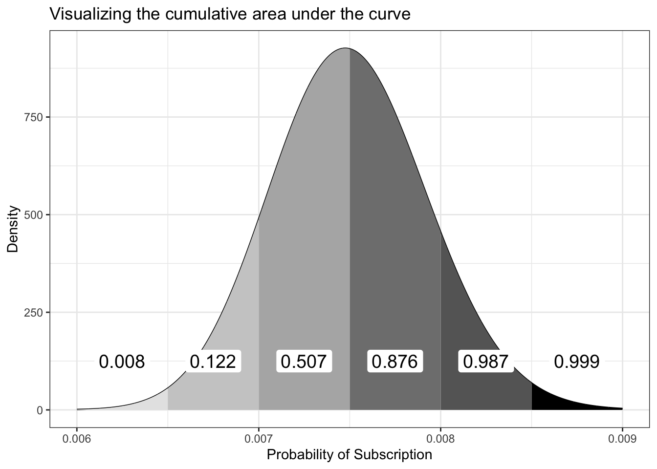
The CDF gets this probability by taking the cumulative area under the curve for the PDF (for those comfortable with calculus, the CDF is the anti-derivative of the PDF). We can summarize this process in two steps: (1) figure out the cumulative area under the curve for each value of the PDF, and (2) plot those values. That’s our CDF.
Figure 13.2: Visualizing the cumulative area under the curve
Figure 13.2 shows the cumulative area under the curve for the PDF of Beta(300,39700). As you can see, our cumulative area under the curve takes into account all of the area in the pieces to its left.
Using this approach, as we move along the PDF, we take into account an increasingly higher probability until our total area is 1, or complete certainty. To turn this into the CDF, we can imagine a function that looks at only these areas under the curve.
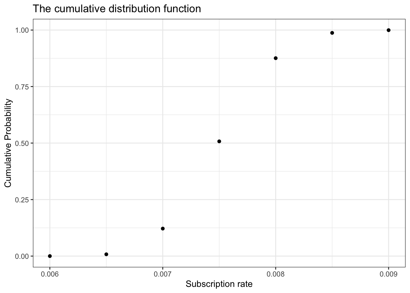
Figure 13.3 shows what happens if we plot the area under the curve for each of our points, which are 0.0005 apart.
Figure 13.3: Plotting just the cumulative probability from Figure 13.2
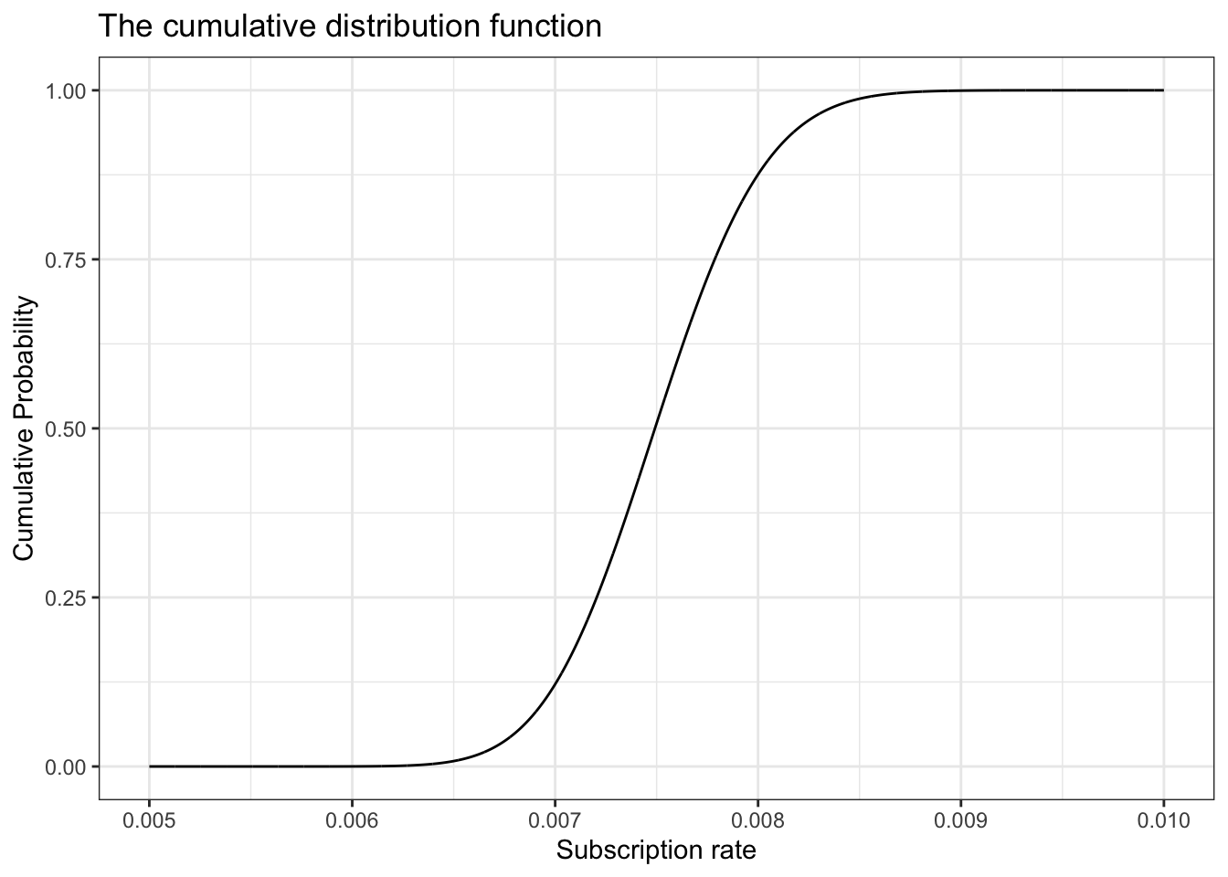
Now we have a way of visualizing just how the cumulative area under the curve changes as we move along the values for our PDF. Of course, the problem is that we’re using these discrete chunks. In reality, the CDF just uses infinitely small pieces of the PDF, so we get a nice smooth line as seen in Figure 13.4.
Figure 13.4: The CDF for our problem
13.3.1 Visualizing and Interpreting the CDF
The PDF is most useful visually for quickly estimating where the peak of a distribution is, and for getting a rough sense of the width (variance) and shape of a distribution. However, with the PDF it is very difficult to reason about the probability of various ranges visually. The CDF is a much better tool for this.
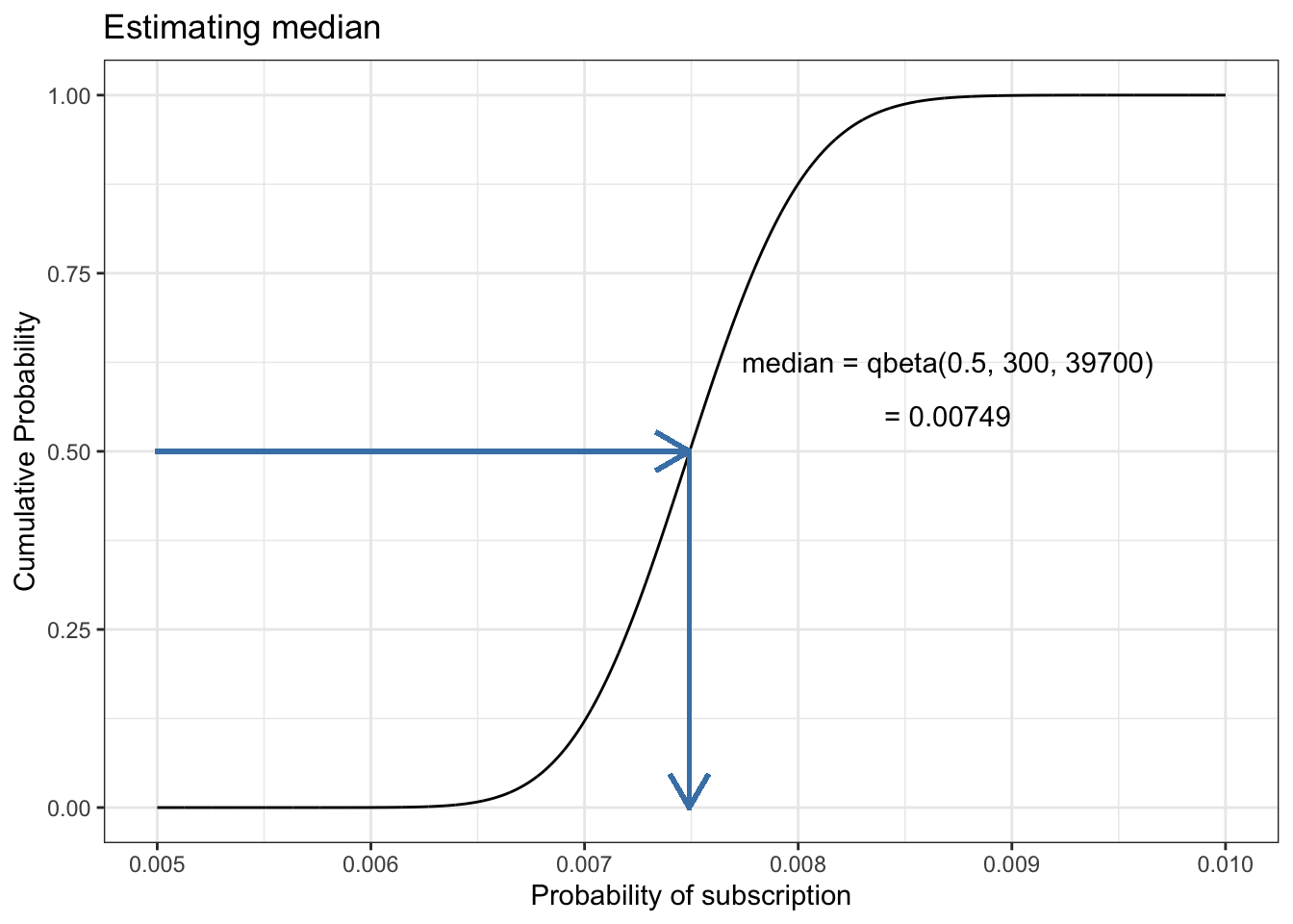
13.3.1.1 Finding the median
Unlike the mean, computing the median can actually be pretty tricky. For small, discrete cases, it’s as simple as putting your observations in order and selecting the value in the middle. But for continuous distributions like our beta distribution, it’s a little more complicated.
Thankfully, we can easily spot the median on a visualization of the CDF. We can simply draw a line from the point where the cumulative probability is 0.5, meaning 50 percent of the values are below this point and 50 percent are above.
Note
There are many packages about the beta functions out there that provides functions for parameter calculation: For instance betamedian() of {betafunctions}. But in a StackOverflow post is the suggestion simple to use qbeta() with p = 0.5.
Figure 13.5: Estimating the median visually using the CDF
13.3.1.2 Approximating Integrals Visually
When working with ranges of probabilities, we’ll often want to know the probability that the true value lies somewhere between some value y and some value x.
Time-consuming computation the integration with R is not necessary as we can eyeball whether or not a certain range of values has a very high probability or a very low probability of occurring.
Figure 13.6: Visually performing integration using the CDF
13.3.1.3 Estimating Confidence Intervals
Looking at the probability of ranges of values leads us to a very important concept in probability: the confidence interval. A confidence interval is a lower and upper bound of values, typically centered on the mean, describing a range of high probability, usually 95, 99, or 99.9 percent. When we say something like “The 95 percent confidence interval is from 12 to 20,” what we mean is that there is a 95 percent probability that our true measurement is somewhere between 12 and 20. Confidence intervals provide a good method of describing the range of possibilities when we’re dealing with uncertain information.
In spite of a special note “In Bayesian statistics what we are calling a ”confidence interval” can go by a few other names, such as ”critical region” or ”critical interval.” In some more traditional schools of statistics, ”confidence interval” has a slightly different meaning, which is beyond the scope of this book.” this concept and notions are not correct for Bayesian statistics. At least what I have learned reading other books, especially (McElreath 2020).
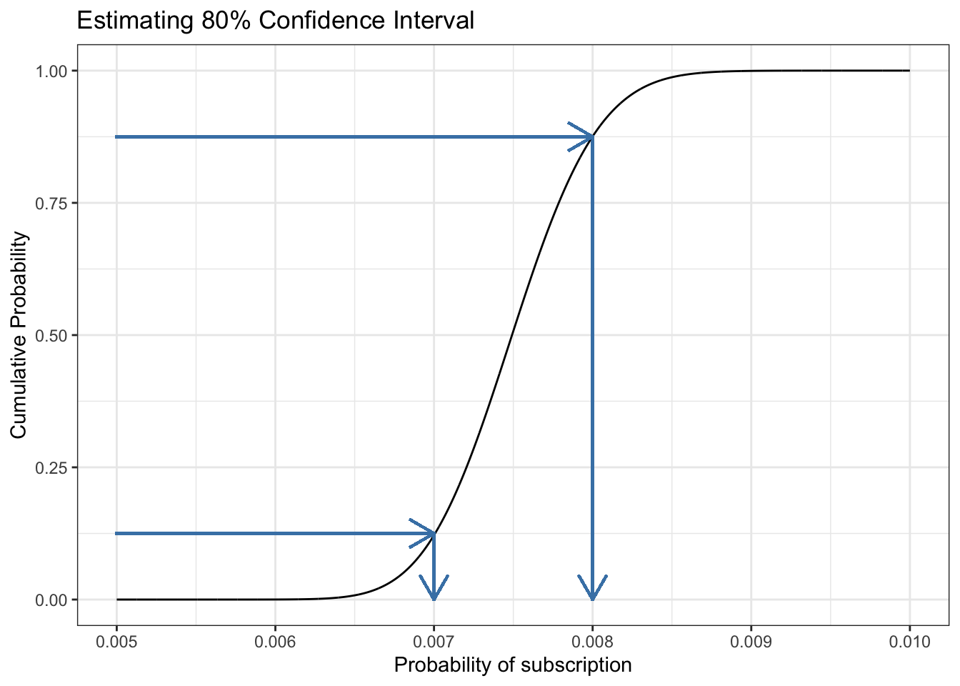
Say we wanted to know the range that covers 80 percent of the possible values for the true conversion rate. We solve this problem by combining our previous approaches: we draw lines at the y-axis from 0.1 and 0.9 to cover 80 percent, and then simply see where on the x-axis these intersect with our CDF:
Figure 13.7: Estimating our confidence intervals visually using the CDF
13.3.2 Using the CDF in R
Just as nearly all major PDFs have a function starting with \(d\), like dnorm(), CDF functions start with \(p\), such as pnorm().
Note
This is a new information for me. Now I understand better the differences and use cases of the different types of distribution. My comprehension will be fostered with the next section when the application of function starting with \(q\) is explained.
Listing 13.5: Calculate the probability that Beta(300,39700) is less than 0.0065
The great thing about CDFs is that it doesn’t matter if your distribution is discrete or continuous. If we wanted to determine the probability of getting three or fewer heads in five coin tosses, for example, we would use the CDF for the binomial distribution like this:
Listing 13.7: Calculate the probability of getting three or fewer heads in five coin tosses
Mathematically, the CDF is like any other function in that it takes an \(x\) value, often representing the value we’re trying to estimate, and gives us a \(y\) value, which represents the cumulative probability. But there is no obvious way to do this in reverse; that is, we can’t give the same function a \(y\) to get an \(x\).
But we did reversing the function when we estimated the median in Section 13.3.1.1 respectively in my version in Section 13.7.5.
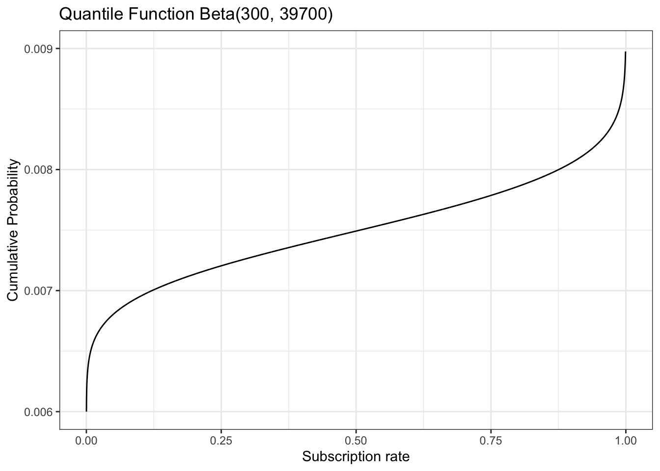
The inverse of the CDF is an incredibly common and useful tool called the quantile function. To compute an exact value for our median and confidence interval, we need to use the quantile function for the beta distribution.
13.4.1 Visualizing and Understanding the Quantile Function
Because the quantile function is simply the inverse of the CDF, it just looks like the CDF rotated 90 degrees, as shown in Figure 13.8.
Figure 13.8: Visually, the quantile function is just a rotation of the CDF
Whenever you hear phrases like:
“The top 10 percent of students …”
“The bottom 20 percent of earners earn less than …”
“The top quartile has notably better performance than …”
you’re talking about values that are found using the quantile function
For example, if we want to know the value that 99.9 percent of the distribution is less than, we can use qbeta() with the quantile we’re interested in calculating as the first argument, and the alpha and beta parameters of our beta distribution as the second and third arguments, like so:
Listing 13.8: Value that we 99.9 percent certain that the true conversion rate for our emails is less than 0.0089
The result is 0.0089, meaning we can be 99.9 percent certain that the true conversion rate for our emails is less than 0.0089.
With the quantile function we can also calculate the 95% confidence interval by finding the lower and upper 2.5% quantile:
Listing 13.9: Calculate the 95% confidence interval
glue::glue("The lower bound is {round(qbeta(0.025,300,39700), 7)} and the upper bound is {round(qbeta(0.975,300,39700) ,7)}.")
#> The lower bound is 0.0066781 and the upper bound is 0.0083686.
Now we can confidently say that we are 95 percent certain that the real conversion rate for blog visitors is somewhere between 0.67 percent and 0.84 percent. … Suppose an article on your blog goes viral and gets 100,000 visitors. Based on our calculations, we know that we should expect between 670 and 840 new email subscribers.
13.5 Wrapping Up
13.6 Exercises
Try answering the following questions to see how well you understand the tools of parameter estimation. The solutions can be found at https://nostarch.com/learnbayes/.
13.6.1 Exercise 13-1
Using the code example for plotting the PDF on page 127, plot the CDF and quantile functions.
Returning to the task of measuring snowfall from Chapter 10, say you have the following measurements (in inches) of snowfall: 7.8, 9.4, 10.0, 7.9, 9.4, 7.0, 7.0, 7.1, 8.9, 7.4
What is your 99.9 percent confidence interval for the true value of snowfall?
Listing 13.10: Calculate the 99% confidence interval
x<-c(7.8, 9.4, 10.0, 7.9, 9.4, 7.0, 7.0, 7.1, 8.9, 7.4)glue::glue("The lower bound is {round(qnorm(0.0005,mean(x), sd(x)), 2)} and the upper bound is {round(qnorm(0.9995,mean(x), sd(x)), 2)}.")
#> The lower bound is 4.46 and the upper bound is 11.92.
Warning
Besides that in my try I used the sd_fun() function from Listing 12.3, I commit an error in using bounds of 0.001 and 0.999 instead of 0.0005 and 0.9995.
13.6.3 Exercise 13-3
A child is going door to door selling candy bars. So far she has visited 30 houses and sold 10 candy bars. She will visit 40 more houses today. What is the 95 percent confidence interval for how many candy bars she will sell the rest of the day?
Listing 13.11: Calculate the 95 percent confidence interval for how many candy bars will be sold
glue::glue("The lower bound is {round(qbeta(0.025, 10, 20), 2)}% and the upper bound is {round(qbeta(0.975, 10, 20), 2)}%.")
#> The lower bound is 0.18% and the upper bound is 0.51%.
Listing 13.12: Calculate the 95 percent confidence interval for how many candy bars will be sold
glue::glue("This means that she will with 95% probability get between 40 * 0.18 = {40 * 0.18} and 40 * 0.51 = {40 * 0.51} candy bars.")
#> This means that she will with 95% probability get between 40 * 0.18 = 7.2 and 40 * 0.51 = 20.4 candy bars.
Listing 13.13: Calculate the 95 percent confidence interval for how many candy bars will be sold
glue::glue("But she can only sell complete bars: Therefore she will sell between {floor(40 * 0.18)} and {floor(40 * 0.51)} candy bars.")
#> But she can only sell complete bars: Therefore she will sell between 7 and 20 candy bars.
13.7 Experiments
I started with Figure 13.13 because this is the easiest graph, as it replicates Figure 13.4 with just the CDF and nothing else. So maybe you will begin also with this basic plot. After Figure 13.13 the natural sequence – ordered by complexity – is Figure 13.12. After that you can inspect in detail my different tries with Figure 13.2 (Figure 13.9, Figure 13.10 and my best solution Figure 13.11) . Then follow my sequences here from Figure 13.5 to Figure 13.8.
Important
There is the following system in using distributions with R, exemplified with the normal distribution:
dnorm for plotting probability densities functions (PDFs).
pnorm for plotting cumulative distribution functions (CDFs).
qnorm for plotting quantile functions, it is the reverse of CDFs.
rnorm for generating and plotting random distributions.
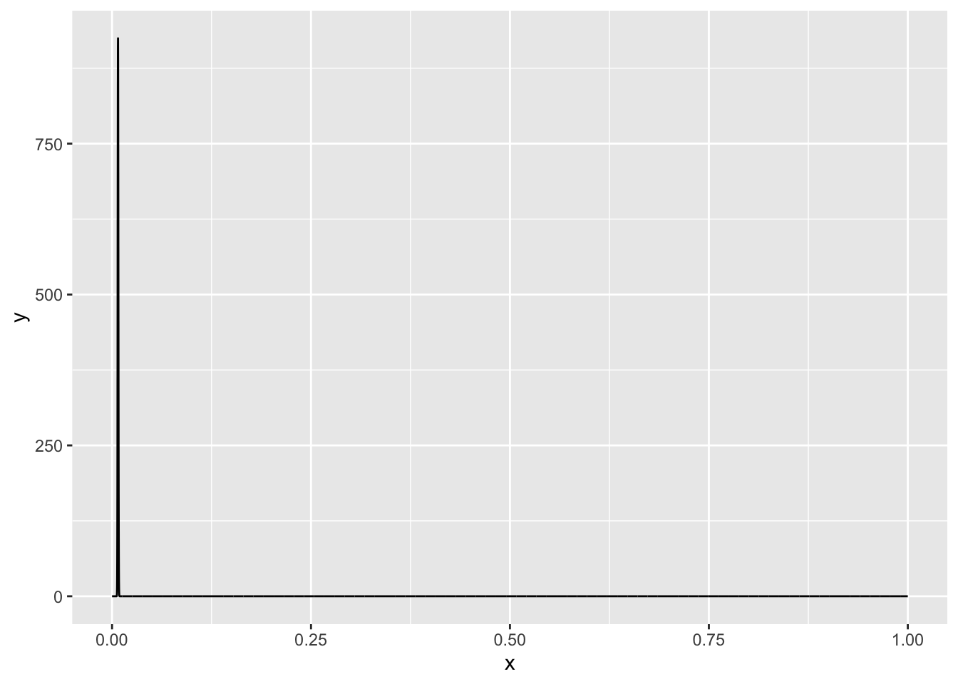
The problem here is that the interesting part of the PDF is very small as we know from the \(\frac{300}{40000} = 0.0075\). Therefore it does not make sense to spread the grid from 0 to 1. We get a much better visualization in the area 0 to 001:
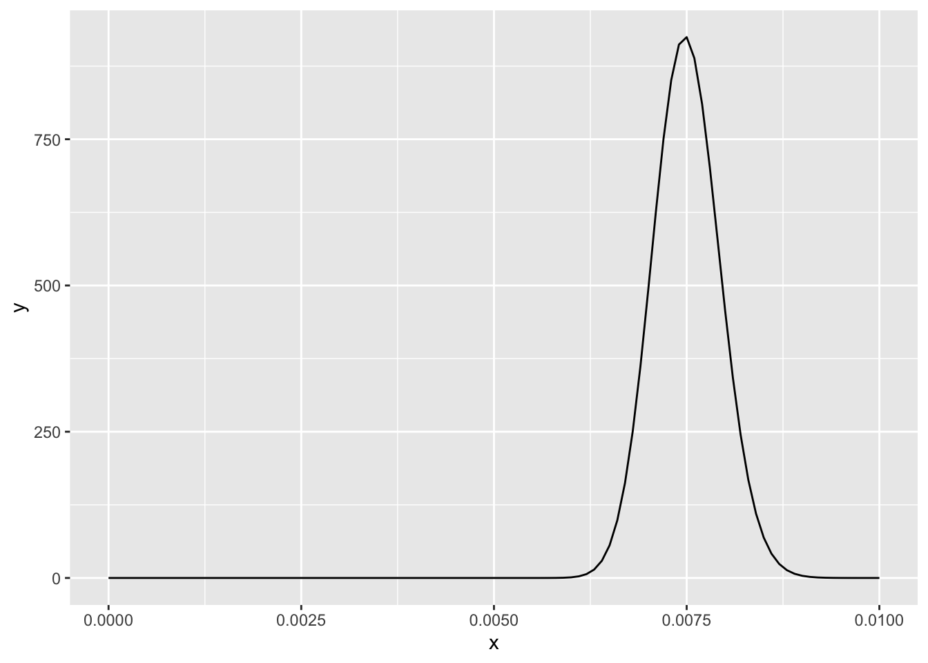
13.7.1.2 Better dimension of x-axis but still not identical for Figure 13-1
But even this curve is not optimal. Now let’s try the interval [0.005, 0.01]:
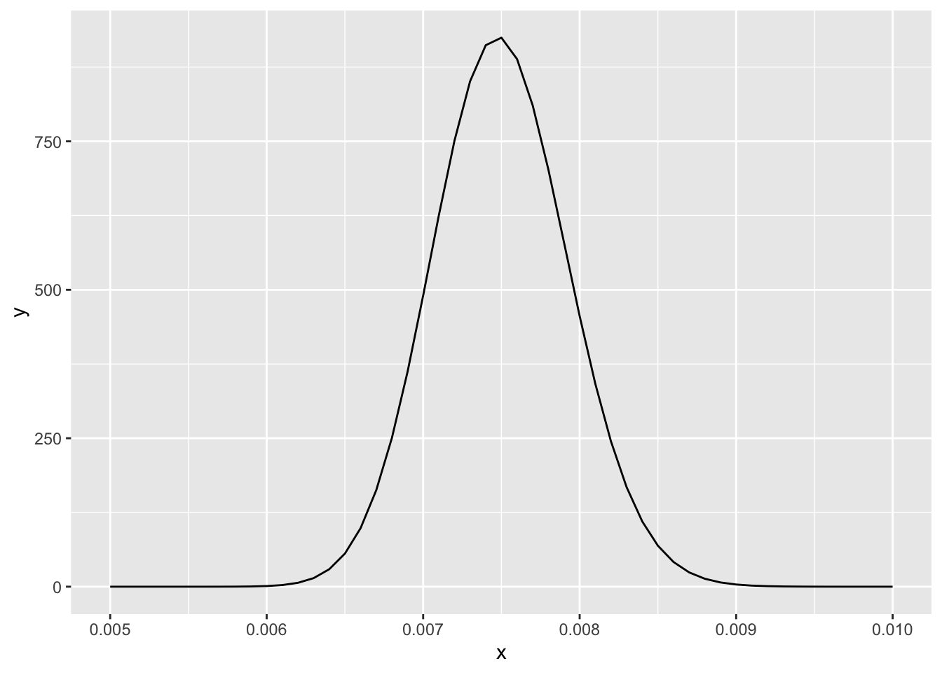
13.7.1.3 Optimal dimension of x-axis but grid too wide for smooth Figure 13-1
tibble::tibble(x =seq(0.005, 0.01, .0001), y =dbeta(x, 300, 39700))|>ggplot2::ggplot(ggplot2::aes(x =x, y =y))+ggplot2::geom_line()
It turns out that this is the interval also used in the book example. But in my visualization you can see some irregularity at the top, because my grid has too coarse. It has only 51 values. Let’s try a much finer grid with 5001 values:
13.7.1.4 Optimal replication of Figure 13-1
tibble::tibble(x =seq(0.005, 0.01, .00001), y =dbeta(x, 300, 39700))|>ggplot2::ggplot(ggplot2::aes(x =x, y =y))+ggplot2::geom_line()
13.7.2 Replicate Figure 13-2
13.7.2.1 First try (bad)
Note
I had to learn about the difference between annotate(geom = "text" …) and annotate(geom = "label" …). There are two big differences:
geom_text() does not understand the fill aesthetics, e.g. you can’t change the background color of the text.
geom_label() “is considerable slower than geom_text()” and does not support the check_overlap argument and the angle aesthetic. But more important for my use case geom_label() draws a rectangle around the label. You need to add label.size = NA to remove the label. Although the option label.size is documented (“Size of label border, in mm.”) using NA to remove the border completely is not explained. I had to find out it the hard way via StackOverflow.
Listing 13.14: Highlighting the cumulative area under the curve
x_lower<-seq(0.006, 0.0085, 0.0005)x_upper<-seq(0.0065, 0.009, 0.0005)text_pos<-seq(0.00625, 0.00875, 0.0005)colors<-c("gray90", "gray80", "gray70", "gray50", "gray40", "black")df_13_2<-tibble::tibble(x =seq(0.006, 0.009, length.out =6000), y =dbeta(x, 300, 39700))ggplot2::ggplot(df_13_2, ggplot2::aes(x =x, y =y))+ggplot2::geom_line()+ggplot2::geom_area(data =df_13_2|>dplyr::filter(x>=x_lower[1]&x<x_upper[1]), fill =colors[1])+ggplot2::annotate(geom ="label", x =text_pos[1], size =5, y =125, color ="black", fill ="white", label.size =NA, label =round(integrate(function(x)dbeta(x, 300, 39700), x_lower[1], x_upper[1])[["value"]], 3))+ggplot2::geom_area(data =df_13_2|>dplyr::filter(x>=x_lower[2]&x<x_upper[2]), fill =colors[2])+ggplot2::annotate(geom ="label", x =text_pos[2], size =5, y =125, color ="black", fill ="white", label.size =NA, label =round(integrate(function(x)dbeta(x, 300, 39700), x_lower[1], x_upper[2])[["value"]], 3))+ggplot2::geom_area(data =df_13_2|>dplyr::filter(x>=x_lower[3]&x<x_upper[3]), fill =colors[3])+ggplot2::annotate(geom ="label", x =text_pos[3], size =5, y =125, color ="black", fill ="white", label.size =NA, label =round(integrate(function(x)dbeta(x, 300, 39700), x_lower[1], x_upper[3])[["value"]], 3))+ggplot2::geom_area(data =df_13_2|>dplyr::filter(x>=x_lower[4]&x<x_upper[4]), fill =colors[4])+ggplot2::annotate(geom ="label", x =text_pos[4], size =5, y =125, color ="black", fill ="white", label.size =NA, label =round(integrate(function(x)dbeta(x, 300, 39700), x_lower[1], x_upper[4])[["value"]], 3))+ggplot2::geom_area(data =df_13_2|>dplyr::filter(x>=x_lower[5]&x<x_upper[5]), fill =colors[5])+ggplot2::annotate("label", x =text_pos[5], size =5, y =125, color ="black", fill ="white", label.size =NA, label =round(integrate(function(x)dbeta(x, 300, 39700), x_lower[1], x_upper[5])[["value"]], 3))+ggplot2::geom_area(data =df_13_2|>dplyr::filter(x>=x_lower[6]&x<x_upper[6]), fill =colors[6])+ggplot2::annotate(geom ="label", x =text_pos[6], size =5, y =125, color ="black", fill ="white", label.size =NA, label =round(integrate(function(x)dbeta(x, 300, 39700), x_lower[1], x_upper[6])[["value"]], 3))+ggplot2::theme_bw()+ggplot2::labs( title ="Visualizing the cumulative area under the curve", x ="Probability of Subscription", y ="Density")
Figure 13.9: Visualizing the cumulative area under the curve
13.7.2.2 Second try (Slightly better)
Warning
I am very unhappy about the many duplicates of Listing 13.14. I tried to use loops or vectorized commands but the best I found out is Listing 13.15 with has still six duplicate code lines.
Listing 13.15: Highlighting the cumulative area under the curve
x_lower<-seq(0.006, 0.0085, 0.0005)x_upper<-seq(0.0065, 0.009, 0.0005)label_x_pos<-seq(0.00625, 0.00875, 0.0005)colors<-c("gray90", "gray80", "gray70", "gray50", "gray40", "black")cum_rate=0for(iin1:6){cum_rate[i]<-round(integrate(function(x)dbeta(x, 300, 39700), x_lower[1], x_upper[i])[["value"]], 3)}add_label<-function(x_pos, txt){ggplot2::annotate( geom ="label", x =x_pos, y =125, size =5, label =txt, label.size =NA)}highlight_one_area<-function(df, i){ggplot2::geom_area(data =df|>dplyr::filter(x>=x_lower[i]&x<x_upper[i]), fill =colors[i])}df_13_2<-tibble::tibble(x =seq(0.006, 0.009, length.out =6000), y =dbeta(x, 300, 39700))p_13_2<-ggplot2::ggplot(df_13_2, ggplot2::aes(x =x, y =y))+ggplot2::geom_line()+highlight_one_area(df_13_2, 1)+highlight_one_area(df_13_2, 2)+highlight_one_area(df_13_2, 3)+highlight_one_area(df_13_2, 4)+highlight_one_area(df_13_2, 5)+highlight_one_area(df_13_2, 6)+add_label(label_x_pos, cum_rate)+ggplot2::theme_bw()+ggplot2::labs( title ="Visualizing the cumulative area under the curve", x ="Probability of Subscription", y ="Density")p_13_2
Figure 13.10: Visualizing the cumulative area under the curve
13.7.2.3 Third try (My best version)
As I could not find a better solution for Listing 13.15 myself I posted my question in StackOverflow and got an answer with two different options within one hour!
The first solution is to use lapply(). I should have known that as I came over a similar solution. The second solution is for me more complex and I have still to study it thoroughly to understand it.
What follows in Listing 13.16 is the modern take of lapply() using the purrr::map() function. (I do not understand why I had to use exactly the argument “df” and asked via SO comment.)
Listing 13.16: Highlighting the cumulative area under the curve
########### Vectors ##############x_lower<-seq(0.006, 0.0085, 0.0005)x_upper<-seq(0.0065, 0.009, 0.0005)label_x_pos<-seq(0.00625, 0.00875, 0.0005)colors<-c("gray90", "gray80", "gray70", "gray50", "gray40", "black")########### Functions ############cum_rate=0for(iin1:6){cum_rate[i]<-round(integrate(function(x)dbeta(x, 300, 39700), x_lower[1], x_upper[i])[["value"]], 3)}add_label<-function(x_pos, txt){ggplot2::annotate( geom ="label", x =x_pos, y =125, size =5, label =txt, label.size =NA)}highlight_areas<-function(df, i){ggplot2::geom_area(data =df|>dplyr::filter(x>=x_lower[i]&x<x_upper[i]), fill =colors[i])}######### Graph plotting ############df_13_2<-tibble::tibble(x =seq(0.006, 0.009, length.out =6000), y =dbeta(x, 300, 39700))p_13_2<-ggplot2::ggplot(df_13_2, ggplot2::aes(x =x, y =y))+ggplot2::geom_line()+purrr::map(1:6, highlight_areas, df =df_13_2)+add_label(label_x_pos, cum_rate)+ggplot2::theme_bw()+ggplot2::labs( title ="Visualizing the cumulative area under the curve", x ="Probability of Subscription", y ="Density")p_13_2
Figure 13.11: Visualizing the cumulative area under the curve
13.7.3 Replicate Figure 13-3
Listing 13.17: Plot the cumulative area under the curve
df_13_3<-tibble::tibble(x =seq(0.006, 0.009, 0.0005), y =pbeta(x, 300, 39700))ggplot2::ggplot(df_13_3, ggplot2::aes(x =x, y =y))+ggplot2::geom_point()+ggplot2::theme_bw()+ggplot2::labs( title ="The cumulative distribution function", x ="Subscription rate", y ="Cumulative Probability")
Figure 13.12: Plotting just the cumulative probability from Figure 13-2
13.7.4 Replicate Figure 13-4
13.7.4.1 Cumulative Distribution Function (CDF)
Listing 13.18: Plot the Cumulative Distribution Function (CDF)
df_13_4a<-tibble::tibble(x =seq(0.005, 0.01, 1e-6), y =pbeta(x, 300, 39700))ggplot2::ggplot(df_13_4a, ggplot2::aes(x =x, y =y))+ggplot2::geom_line()+ggplot2::theme_bw()+ggplot2::labs( title ="The cumulative distribution function", x ="Subscription rate", y ="Cumulative Probability")
Figure 13.13: The CDF for our problem
13.7.4.2 Empiricial Cumulative Distribution Function (ECDF) - with steps
Note
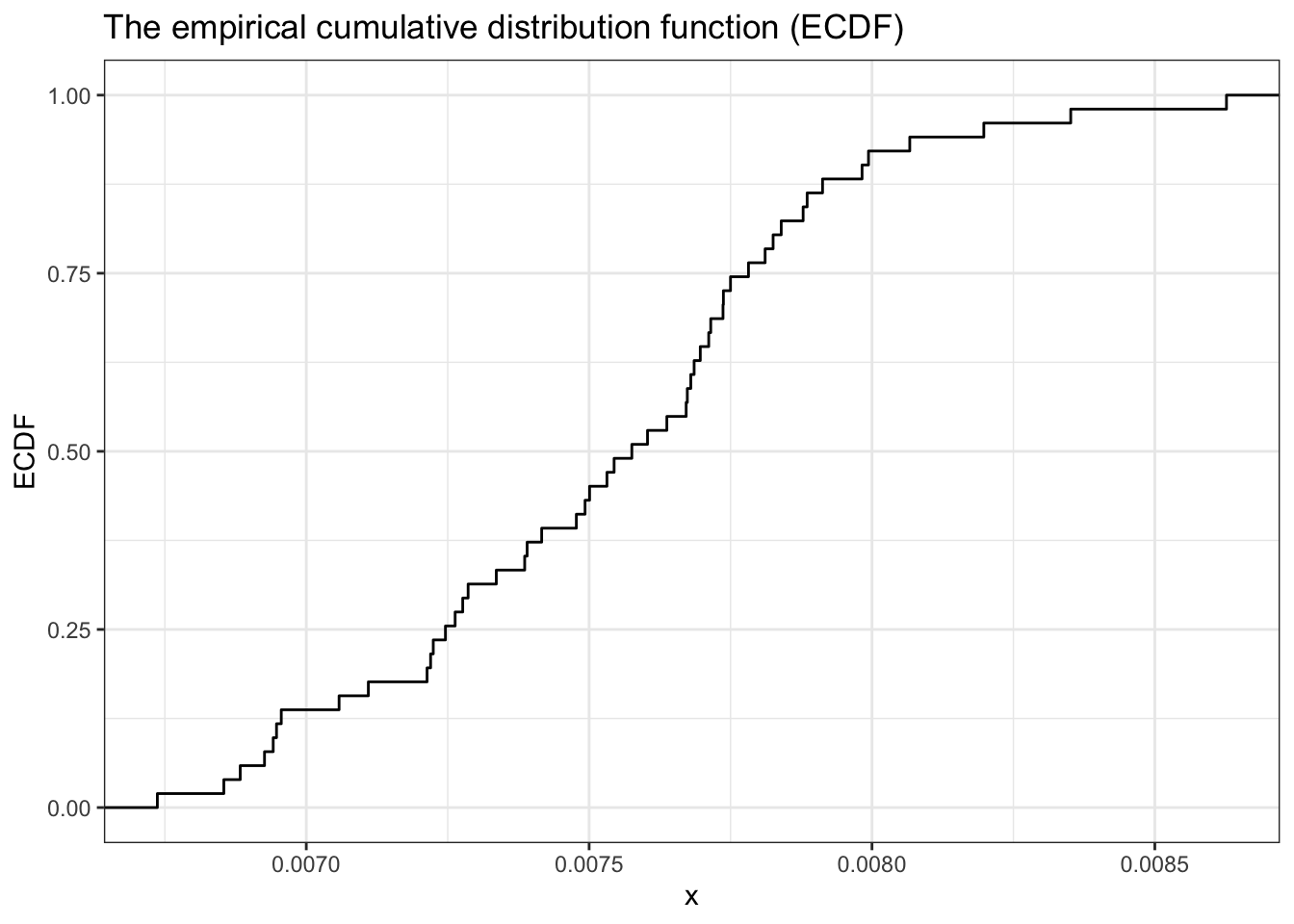
Trying to apply the CDF I noticed that there is also an rglossary(“ECDF”)` (Empirical Cumulative Distribution Function). The differences are that the ECDF is a step function whereas the CDF is smooth. But with many different values the ECDF approximates to ta smooth function.
Listing 13.19: Plot the Empirical Cumulative Distribution Function (ECDF)
df_13_4b<-tibble::tibble(x =seq(0.005, 0.01, 1e-4), y =rbeta(x, 300, 39700))ggplot2::ggplot(df_13_4b, ggplot2::aes(y))+ggplot2::stat_ecdf(geom ="step")+ggplot2::theme_bw()+ggplot2::labs( title ="The empirical cumulative distribution function (ECDF)", x ="x", y ="ECDF")
Figure 13.14: The ECDF for our problem
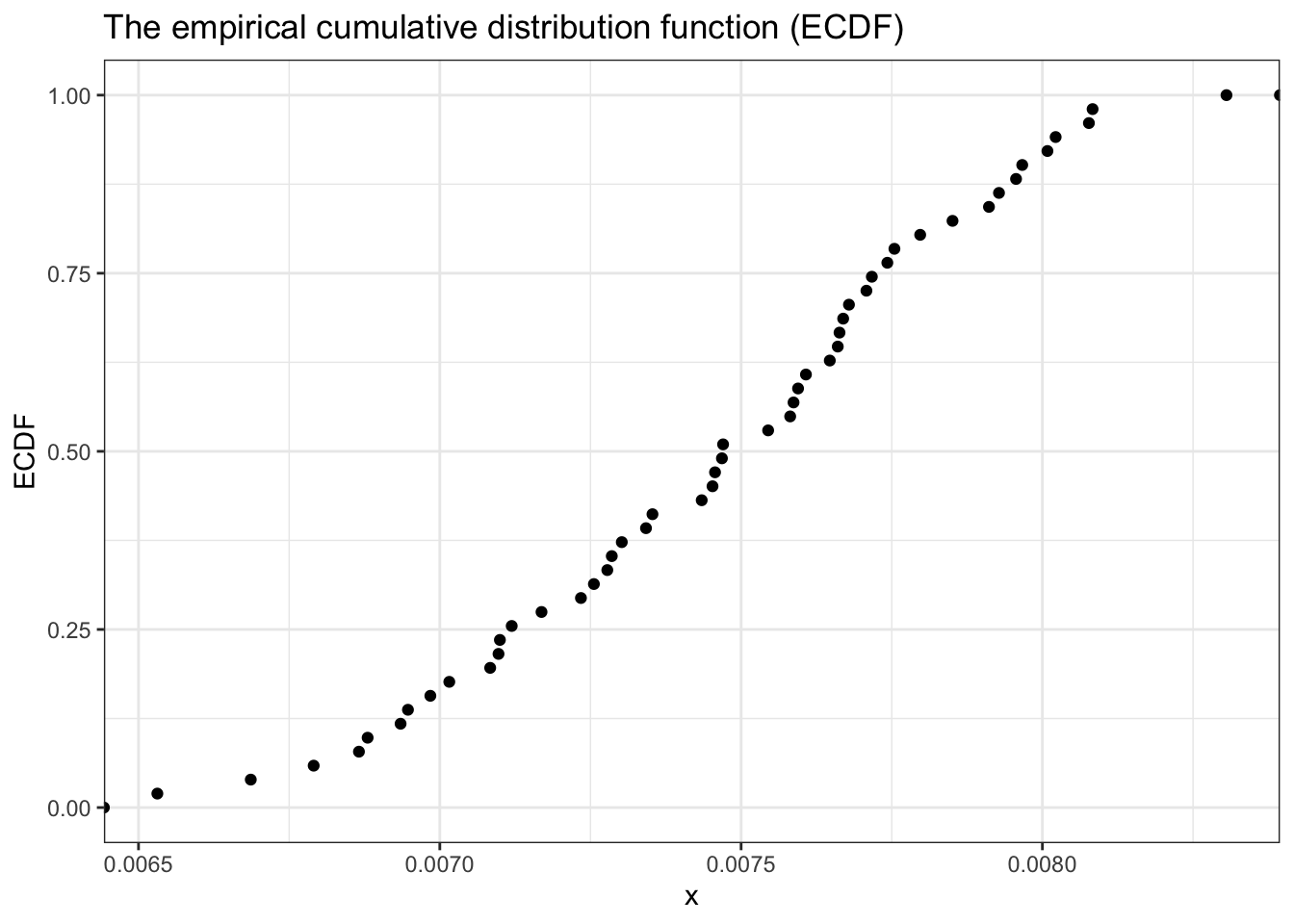
13.7.4.3 Empiricial Cumulative Distribution Function (ECDF) - with points
Listing 13.20: Plot the Cumulative Distribution Function (CDF)
df_13_4c<-tibble::tibble(x =seq(0.005, 0.01, 1e-4), y =rbeta(x, 300, 39700))ggplot2::ggplot(df_13_4c, ggplot2::aes(y))+ggplot2::stat_ecdf(geom ="point")+ggplot2::theme_bw()+ggplot2::labs( title ="The empirical cumulative distribution function (ECDF)", x ="x", y ="ECDF")
Figure 13.15: The ECDF for our problem
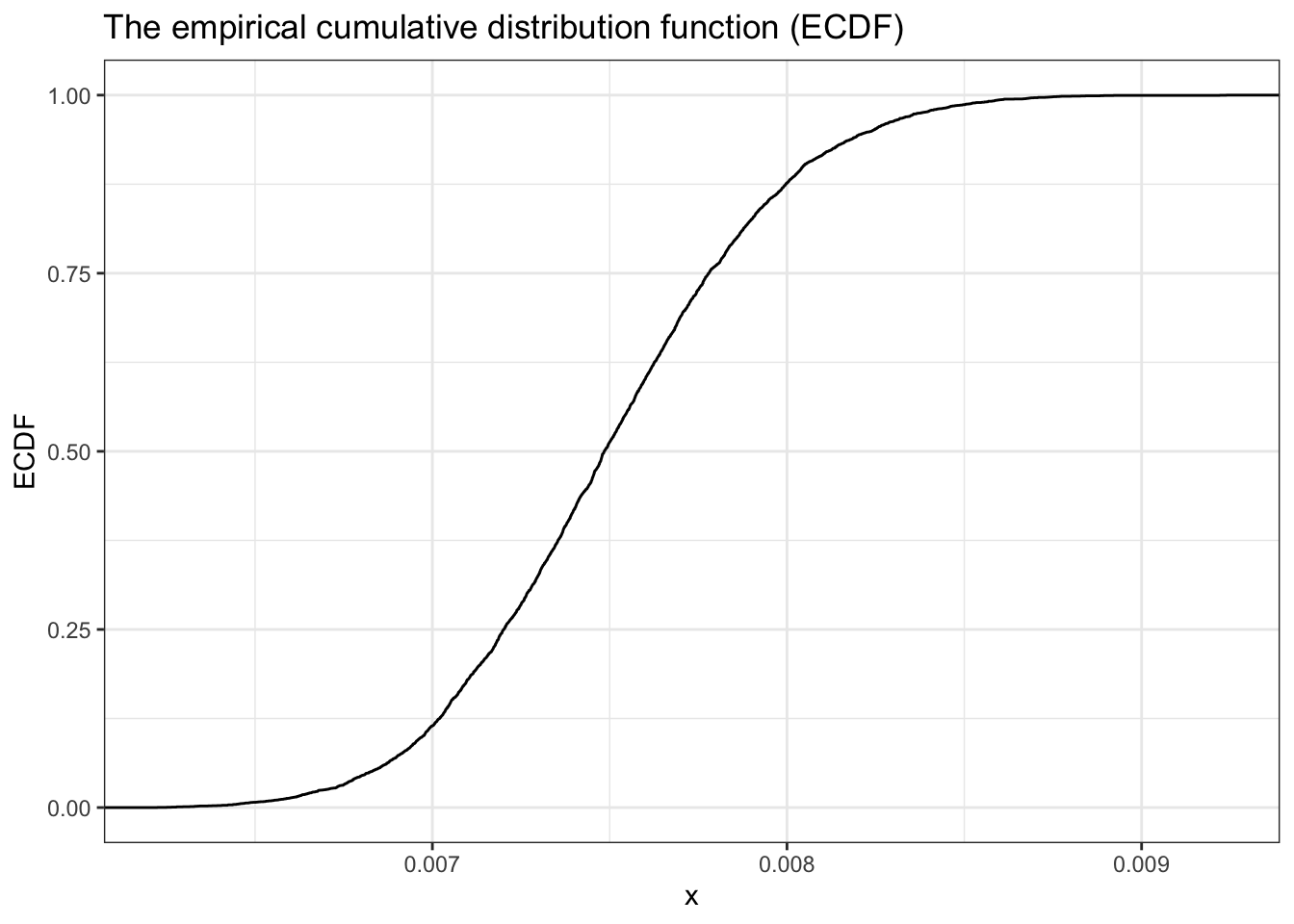
13.7.4.4 Empiricial Cumulative Distribution Function (ECDF) - smooth
Listing 13.21: Plot the Empirical Cumulative Distribution Function (ECDF)
df_13_4d<-tibble::tibble(x =seq(0.005, 0.01, 1e-6), y =rbeta(x, 300, 39700))ggplot2::ggplot(df_13_4d, ggplot2::aes(y))+ggplot2::stat_ecdf(geom ="step")+ggplot2::theme_bw()+ggplot2::labs( title ="The empirical cumulative distribution function (ECDF)", x ="x", y ="ECDF")
Figure 13.16: The ECDF for our problem
13.7.5 Replicate Figure 13-5
Listing 13.22: Estimate and display median using the CDF
median_beta<-round(qbeta(0.5, 300, 39700), 5)df_13_5<-tibble::tibble(x =seq(0.005, 0.01, 1e-6), y =pbeta(x, 300, 39700))ggplot2::ggplot(df_13_5, ggplot2::aes(x =x, y =y))+ggplot2::geom_line()+ggplot2::geom_segment(ggplot2::aes(x =0.005, y =0.50, xend =median_beta, yend =0.50), lineend ="square", linejoin ="bevel", color ="steelblue", size =0.8, arrow =ggplot2::arrow(length =ggplot2::unit(0.5, "cm")))+ggplot2::geom_segment(ggplot2::aes(x =median_beta, y =0.50, xend =median_beta, yend =0.00), lineend ="square", linejoin ="bevel", color ="steelblue", size =0.8, arrow =ggplot2::arrow(length =ggplot2::unit(0.5, "cm")))+ggplot2::annotate("text", y =0.625, x =0.0087, label ="median = qbeta(0.5, 300, 39700)")+ggplot2::annotate("text", y =0.55, x =0.0087, label =glue::glue("= {median_beta}"))+ggplot2::theme_bw()+ggplot2::labs( title ="Estimating median", x ="Probability of subscription", y ="Cumulative Probability")
#> Warning: Using `size` aesthetic for lines was deprecated in ggplot2 3.4.0.
#> ℹ Please use `linewidth` instead.
Figure 13.17: Estimating the median visually using the CDF
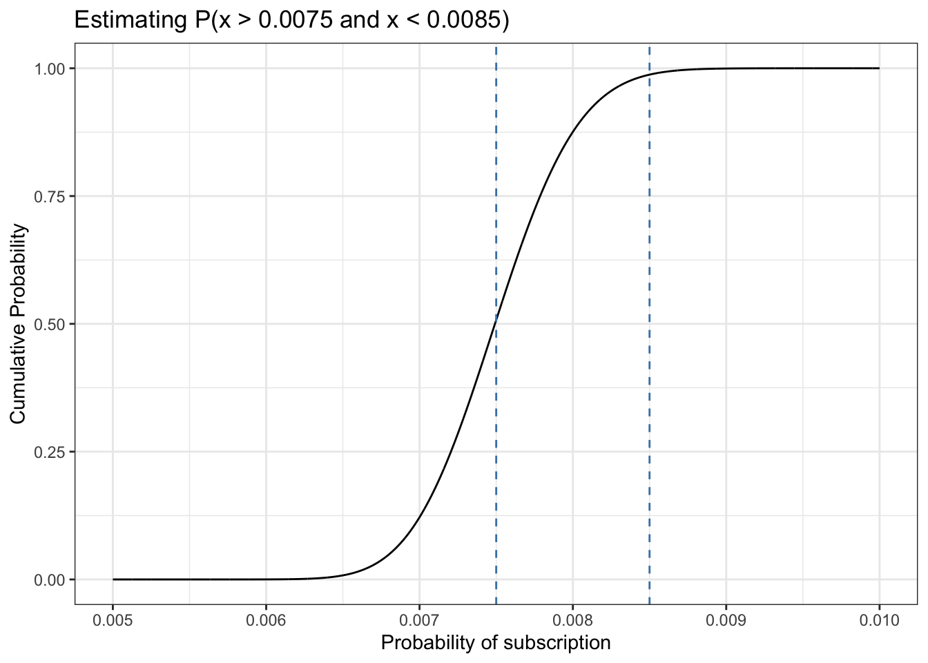
13.7.6 Replicate Figure 13-6
In contrast to Figure 13.17 where I cheated by calculating the median of the beta distribution I will in Section 13.7.6 try to approximate the integration just visually.
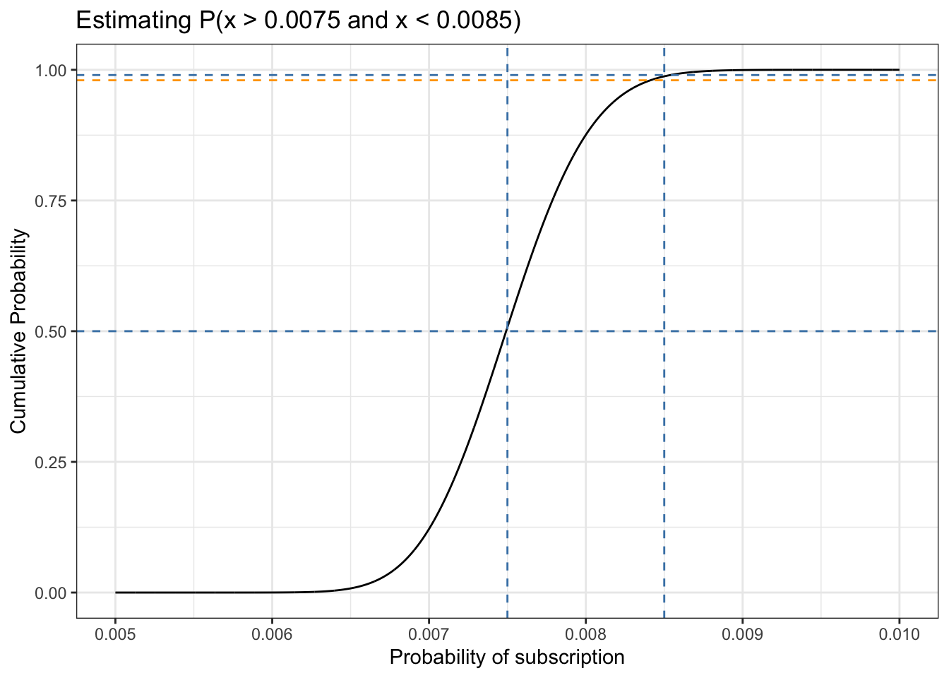
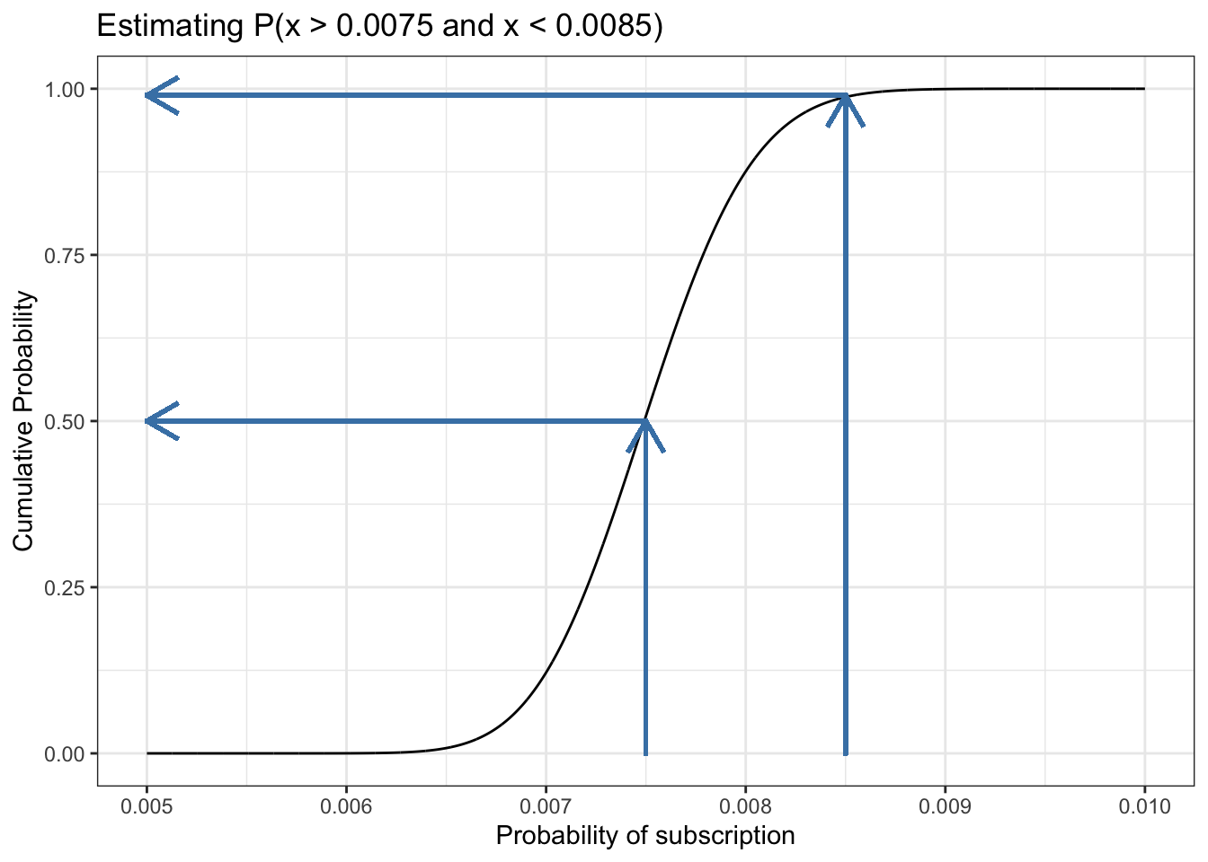
We are going to estimate the range between p(x > 0.0075 and x < 0.0085). The solution could be visually done approximately either with a ruler or (not so exact) just by eyeballing. To do it programmatically without integration is a somewhat complex procedure with four steps:
First I have to draw vertical lines from the start and end of the interesting range. These lines have to cross the CDF because I do not know the value of the cumulative probability where they meet the CDF.
Then I have to inspect the intersection visually and try to estimate and draw the horizontal lines. This has to be done several times until the two lines cross (almost) exactly at the CDF.
Now I can limit the vertical and horizontal lines, so that they stop at the CDF.
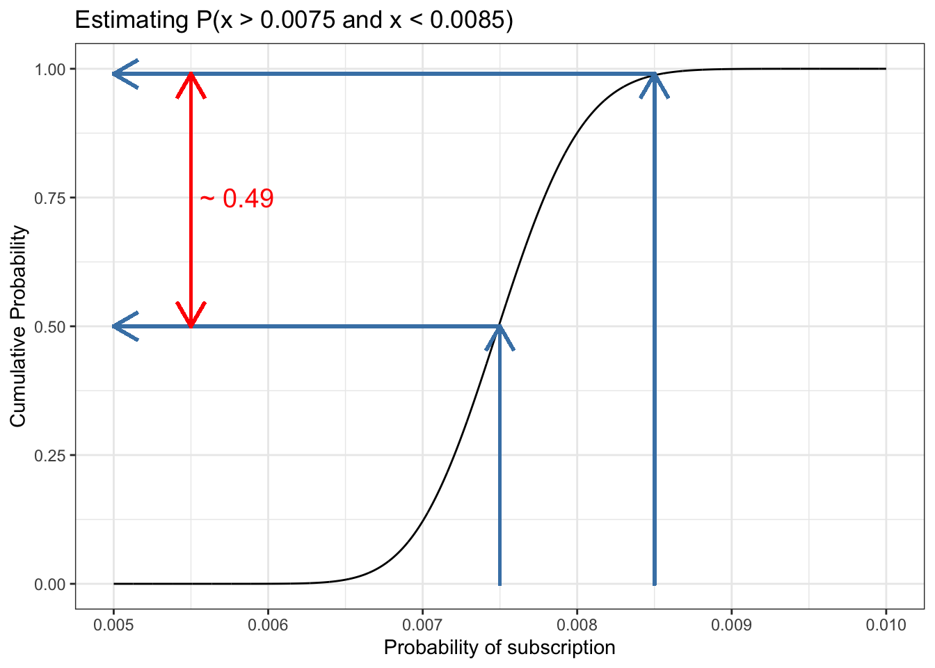
The last step is to estimate the range by reading the intersection at the y-axis.
13.7.6.1 First step
Listing 13.23: Approximate the integration of a range of the CDF: First step
df_13_6<-tibble::tibble(x =seq(0.005, 0.01, 1e-6), y =pbeta(x, 300, 39700))ggplot2::ggplot(df_13_6, ggplot2::aes(x =x, y =y))+ggplot2::geom_line()+ggplot2::geom_vline(xintercept =0.0075, color ="steelblue", linetype ="dashed")+ggplot2::geom_vline(xintercept =0.0085, color ="steelblue", linetype ="dashed")+ggplot2::theme_bw()+ggplot2::labs( title ="Estimating P(x > 0.0075 and x < 0.0085)", x ="Probability of subscription", y ="Cumulative Probability")
Figure 13.18: Visually performing integration using the CDF: First step
13.7.6.2 Second step
The lower cumulative probability is almost exact 0.5 as I can see and already know from Figure 13.17. Without knowing the solution in the book my first approach was to draw a line at 0.98% of the CDF (orange). As this seems a little to less a tried with it .99%
Listing 13.24: Approximate the integration of a range of the CDF: Second step
df_13_6<-tibble::tibble(x =seq(0.005, 0.01, 1e-6), y =pbeta(x, 300, 39700))ggplot2::ggplot(df_13_6, ggplot2::aes(x =x, y =y))+ggplot2::geom_line()+ggplot2::geom_vline(xintercept =0.0075, color ="steelblue", linetype ="dashed")+ggplot2::geom_vline(xintercept =0.0085, color ="steelblue", linetype ="dashed")+ggplot2::geom_hline(yintercept =0.5, color ="steelblue", linetype ="dashed")+ggplot2::geom_hline(yintercept =0.98, color ="orange", linetype ="dashed")+ggplot2::geom_hline(yintercept =0.99, color ="steelblue", linetype ="dashed")+ggplot2::theme_bw()+ggplot2::labs( title ="Estimating P(x > 0.0075 and x < 0.0085)", x ="Probability of subscription", y ="Cumulative Probability")
Figure 13.19: Visually performing integration using the CDF: Second step
13.7.6.3 Third step
Listing 13.25: Approximate the integration of a range of the CDF: Third step
df_13_6<-tibble::tibble(x =seq(0.005, 0.01, 1e-6), y =pbeta(x, 300, 39700))ggplot2::ggplot(df_13_6, ggplot2::aes(x =x, y =y))+ggplot2::geom_line()+ggplot2::geom_segment(ggplot2::aes(xend =0.005, yend =0.50, x =0.00750, y =0.50), lineend ="square", linejoin ="bevel", color ="steelblue", size =0.8, arrow =ggplot2::arrow(length =ggplot2::unit(0.5, "cm")))+ggplot2::geom_segment(ggplot2::aes(xend =0.0075, yend =0.50, x =0.0075, y =0.00), lineend ="square", linejoin ="bevel", color ="steelblue", size =0.8, arrow =ggplot2::arrow(length =ggplot2::unit(0.5, "cm")))+ggplot2::geom_segment(ggplot2::aes(x =0.0085, y =0, xend =0.0085, yend =0.99), lineend ="square", linejoin ="bevel", color ="steelblue", size =0.8, arrow =ggplot2::arrow(length =ggplot2::unit(0.5, "cm")))+ggplot2::geom_segment(ggplot2::aes(x =0.0085, y =0.99, xend =0.005, yend =0.99), lineend ="square", linejoin ="bevel", color ="steelblue", size =0.8, arrow =ggplot2::arrow(length =ggplot2::unit(0.5, "cm")))+ggplot2::theme_bw()+ggplot2::labs( title ="Estimating P(x > 0.0075 and x < 0.0085)", x ="Probability of subscription", y ="Cumulative Probability")
Figure 13.20: Visually performing integration using the CDF: Third step
13.7.6.4 Fourth step
Listing 13.26: Approximate the integration of a range of the CDF: Fourth step
df_13_6<-tibble::tibble(x =seq(0.005, 0.01, 1e-6), y =pbeta(x, 300, 39700))ggplot2::ggplot(df_13_6, ggplot2::aes(x =x, y =y))+ggplot2::geom_line()+ggplot2::geom_segment(ggplot2::aes(xend =0.005, yend =0.50, x =0.00750, y =0.50), lineend ="square", linejoin ="bevel", color ="steelblue", size =0.8, arrow =ggplot2::arrow(length =ggplot2::unit(0.5, "cm")))+ggplot2::geom_segment(ggplot2::aes(xend =0.0075, yend =0.50, x =0.0075, y =0.00), lineend ="square", linejoin ="bevel", color ="steelblue", size =0.8, arrow =ggplot2::arrow(length =ggplot2::unit(0.5, "cm")))+ggplot2::geom_segment(ggplot2::aes(x =0.0085, y =0, xend =0.0085, yend =0.99), lineend ="square", linejoin ="bevel", color ="steelblue", size =0.8, arrow =ggplot2::arrow(length =ggplot2::unit(0.5, "cm")))+ggplot2::geom_segment(ggplot2::aes(x =0.0085, y =0.99, xend =0.005, yend =0.99), lineend ="square", linejoin ="bevel", color ="steelblue", size =0.8, arrow =ggplot2::arrow(length =ggplot2::unit(0.5, "cm")))+ggplot2::geom_segment(ggplot2::aes(x =0.0055, y =0.5, xend =0.0055, yend =0.99), lineend ="square", linejoin ="bevel", color ="red", size =0.8, arrow =ggplot2::arrow(length =ggplot2::unit(0.5, "cm")))+ggplot2::geom_segment(ggplot2::aes(xend =0.0055, yend =0.5, x =0.0055, y =0.99), lineend ="square", linejoin ="bevel", color ="red", size =0.8, arrow =ggplot2::arrow(length =ggplot2::unit(0.5, "cm")))+ggplot2::annotate("text", x =0.0058, y =0.75, label ="~ 0.49", color ="red", size =5)+ggplot2::theme_bw()+ggplot2::labs( title ="Estimating P(x > 0.0075 and x < 0.0085)", x ="Probability of subscription", y ="Cumulative Probability")
Figure 13.21: Visually performing integration using the CDF: Fourth step
13.7.7 Replicate Figure 13-7
There is nothing new for approximating the range that covers 80 percent of the possible values for the true conversion rate. We use the same strategy as in Section 13.7.6 but this time starting from the y-axis:
Listing 13.27: Approximate the confidence interval via the CDF
df_13_7<-tibble::tibble(x =seq(0.005, 0.01, 1e-6), y =pbeta(x, 300, 39700))ggplot2::ggplot(df_13_7, ggplot2::aes(x =x, y =y))+ggplot2::geom_line()+ggplot2::geom_segment(ggplot2::aes(xend =0.007, yend =0.125, x =0.005, y =0.125), lineend ="square", linejoin ="bevel", color ="steelblue", size =0.6, arrow =ggplot2::arrow(length =ggplot2::unit(0.5, "cm")))+ggplot2::geom_segment(ggplot2::aes(xend =0.0080, yend =0.875, x =0.005, y =0.875), lineend ="square", linejoin ="bevel", color ="steelblue", size =0.6, arrow =ggplot2::arrow(length =ggplot2::unit(0.5, "cm")))+ggplot2::geom_segment(ggplot2::aes(x =0.007, y =0.125, xend =0.007, yend =0.0), lineend ="square", linejoin ="bevel", color ="steelblue", size =0.6, arrow =ggplot2::arrow(length =ggplot2::unit(0.5, "cm")))+ggplot2::geom_segment(ggplot2::aes(x =0.008, y =0.875, xend =0.008, yend =0.0), lineend ="square", linejoin ="bevel", color ="steelblue", size =0.6, arrow =ggplot2::arrow(length =ggplot2::unit(0.5, "cm")))+ggplot2::theme_bw()+ggplot2::labs( title ="Estimating 80% Confidence Interval", x ="Probability of subscription", y ="Cumulative Probability")
Figure 13.22: Estimating our confidence intervals visually using the CDF
13.7.8 Replicate Figure 13-8
Listing 13.28: Plot the quantile function
df_13_8<-tibble::tibble(x =seq(0, 1, 1e-4), y =qbeta(x, 300, 39700))ggplot2::ggplot(df_13_8, ggplot2::aes(x =x, y =y))+ggplot2::ylim(0.006, 0.009)+ggplot2::geom_line()+ggplot2::theme_bw()+ggplot2::labs( title ="Quantile Function Beta(300, 39700)", x ="Subscription rate", y ="Cumulative Probability")
Figure 13.23: Visually, the quantile function is just a rotation of the CDF.
McElreath, Richard. 2020. Statistical Rethinking: A Bayesian Course with Examples in R and Stan. 2nd ed. CRC Texts in Statistical Science. Boca Raton: Taylor; Francis, CRC Press. https://doi.org/10.1201/9780429029608.
Source Code
# Tools of Parameter Estimation: The PDF, CDF, and Quantile Function {#sec-chap-13}> This chapter will cover more on the> `r glossary("probability density function")` (PDF); introduce the> `r glossary("cumulative distribution function")` (CDF), which helps us> more easily determine the probability of ranges of values; and> introduce `r glossary("quantile", "quantiles")`, which divide our> probability distributions into parts with equal probabilities. For> example, a *percentile* is a 100-quantile, meaning it divides the> probability distribution into 100 equal pieces. (115)## Estimating the Conversion Rate for an Email Signup List> Say you run a blog and want to know the probability that a visitor to> your blog will subscribe to your email list. In marketing terms,> getting a user to perform a desired event is referred to as the> *conversion event*, or simply a *conversion*, and the probability that> a user will subscribe is the *conversion rate*.> As discussed in @sec-beta-distribution, we would use the beta> distribution to estimate p, the probability of subscribing, when we> know `k`, the number of people subscribed, and `n`, the total number> of visitors. The two parameters needed for the beta distribution are> `α`, which in this case represents the total subscribed (`k`), and> `β`, representing the total not subscribed (`n – k`).## The Probability Density Function> let's say for the first 40,000 visitors, you get 300 subscribers. The> PDF for our problem is the beta distribution where α = 300 and β => 39,700.::: {#thm-mean-beta}#### Computing the mean of the beta distribution$$\begin{align*}\mu_{Beta} = \frac{\alpha}{\alpha + \beta} \\\mu_{Beta} = \frac{300}{300 + 39,700} = 0.0075\end{align*}$$ {#eq-mean-beta}The blog's average conversion rate is simply$\frac{subscribed}{visited}$.:::### Visualizing and Interpreting the PDF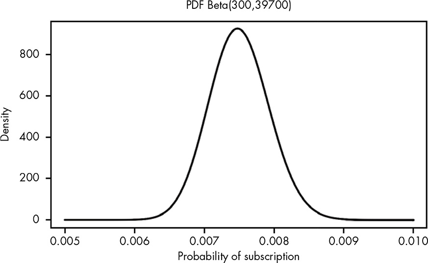{#fig-13-01fig-alt="The beta PDF as almost a normal distribution with mode = mean at .0075"fig-align="center" width="70%"}> Given that we have uncertainty in our measurement, and we have a mean,> it could be useful to investigate how much more likely it is that the> true conversion rate is 0.001 higher or lower than the mean of 0.0075> we observed.```{r}#| label: integrate-higher-lower#| attr-source: '#lst-integrate-higher-lower lst-cap="How much more likely it is that the true conversion rate is 0.001 higher or lower"'integrate(function(x)dbeta(x, 300, 39700), 0, 0.0065)integrate(function(x)dbeta(x, 300, 39700), 0.0085, 1)```> if we had to make a decision with the limited data we have, we could> still calculate how much likelier one extreme is than the other:```{r}#| label: integrate-extremes#| attr-source: '#lst-integrate-extremes lst-cap="How much likelier is one extreme than the other"'integrate(function(x)dbeta(x, 300, 39700), 0.0085, 1)[["value"]] /integrate(function(x)dbeta(x, 300, 39700), 0, 0.0065)[["value"]]```It's 56 percent more likely that our true conversion rate is greaterthan 0.0085 than that it's lower than 0.0065.### Working with the PDF in RI am going to use my own code in @sec-replicate-fig-13-1. But to see what it looks like I use the R base code lines from the book:```{r}#| label: draw-pdf-with-base-r#| attr-source: '#lst-draw-pdf-with-base-r lst-cap="Working with the PDF in base R"'xs <-seq(0.005, 0.01, by =0.00001)xs.all <-seq(0, 1, by =0.0001)plot( xs,dbeta(xs, 300, 40000-300),type ='l',lwd =3,ylab ="density",xlab ="probability of subscription",main ="PDF Beta(300,39700)")```## Introducing the Cumulative Distribution Function> we can save ourselves a lot of effort with the cumulative distribution> function (CDF), which sums all parts of our distribution, replacing a> lot of calculus work. ... The CDF takes in a value and returns the> probability of getting that value or lower.> The CDF gets this probability by taking the cumulative area under the> curve for the PDF (for those comfortable with calculus, the CDF is the> *anti-derivative* of the PDF). We can summarize this process in two> steps: (1) figure out the cumulative area under the curve for each> value of the PDF, and (2) plot those values. That's our CDF.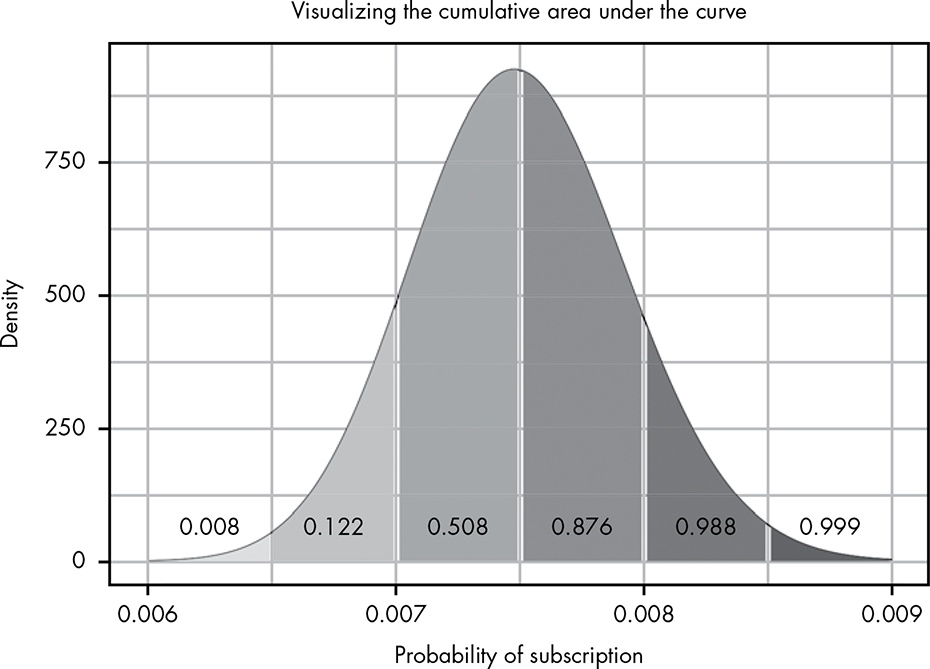{#fig-13-02fig-alt="Visualizing the cumulative area under the curve of the beta distribution in steps to 0.0005"fig-align="center" width="70%"}@fig-13-02 shows the cumulative area under the curve for the PDF ofBeta(300,39700). As you can see, our cumulative area under the curvetakes into account all of the area in the pieces to its left.Using this approach, as we move along the PDF, we take into account anincreasingly higher probability until our total area is 1, or completecertainty. To turn this into the CDF, we can imagine a function thatlooks at only these areas under the curve.@fig-13-03 shows what happens if we plot the area under the curve foreach of our points, which are 0.0005 apart.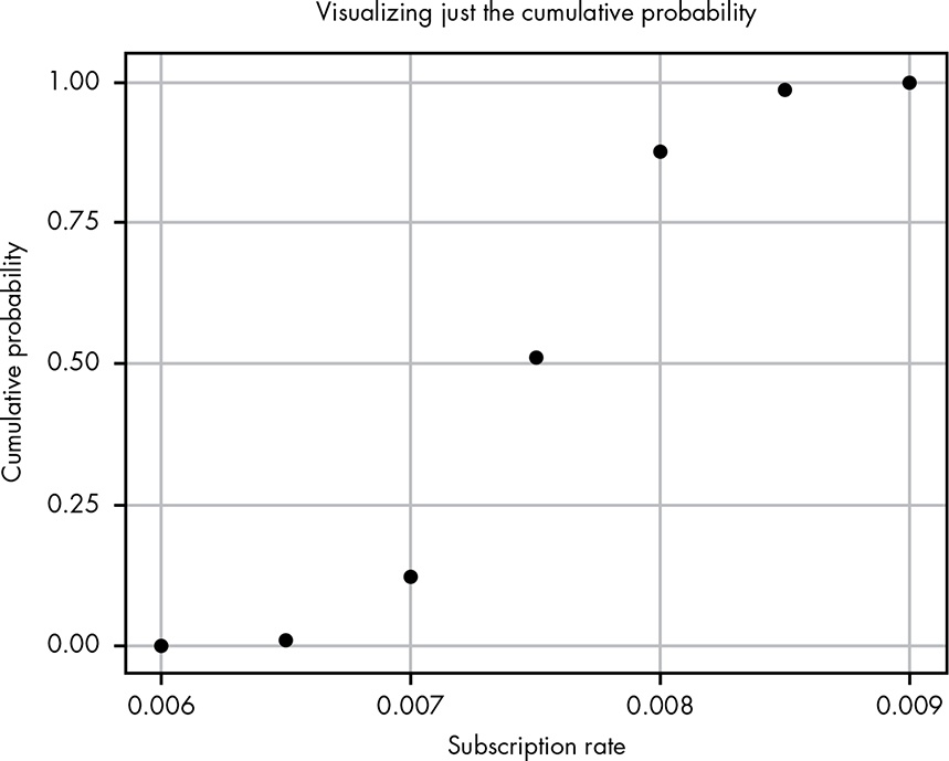{#fig-13-03fig-alt="Plotting the area under the curve for each of our points, which are 0.0005 apart results in an S curve"fig-align="center" width="70%"}> Now we have a way of visualizing just how the cumulative area under> the curve changes as we move along the values for our PDF. Of course,> the problem is that we're using these discrete chunks. In reality, the> CDF just uses infinitely small pieces of the PDF, so we get a nice> smooth line as seen in @fig-13-04.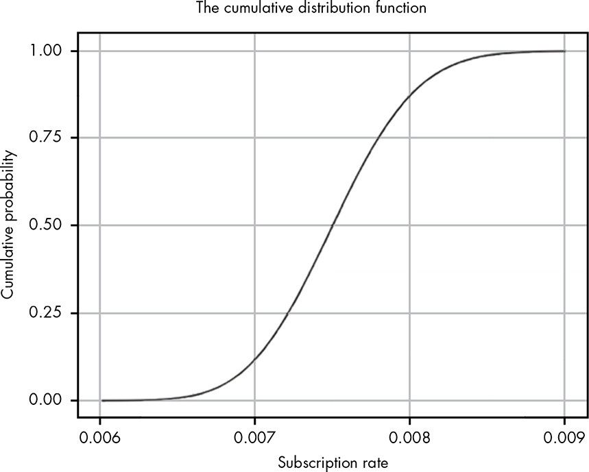{#fig-13-04fig-alt="The CDF for our problem of conversion to blog subscriber"fig-align="center" width="70%"}### Visualizing and Interpreting the CDF> The PDF is most useful visually for quickly estimating where the peak> of a distribution is, and for getting a rough sense of the width> (variance) and shape of a distribution. However, with the PDF it is> very difficult to reason about the probability of various ranges> visually. The CDF is a much better tool for this.#### Finding the median {#sec-finding-the-median}> Unlike the mean, computing the median can actually be pretty tricky.> For small, discrete cases, it's as simple as putting your observations> in order and selecting the value in the middle. But for continuous> distributions like our beta distribution, it's a little more> complicated.> Thankfully, we can easily spot the median on a visualization of the> CDF. We can simply draw a line from the point where the cumulative> probability is 0.5, meaning 50 percent of the values are below this> point and 50 percent are above.::: callout-noteThere are many packages about the beta functions out there that providesfunctions for parameter calculation: For instance `betamedian()` of[{**betafunctions**}](https://search.r-project.org/CRAN/refmans/betafunctions/html/betamedian.html).But in a [StackOverflowpost](https://stackoverflow.com/questions/59077866/is-there-a-way-to-find-the-median-using-beta-distribution-parameters-in-r)is the suggestion simple to use `qbeta()` with `p = 0.5`.This is what I have done in replicating @fig-13-05 with my @fig-pb-13-5.:::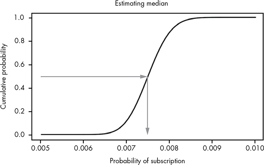{#fig-13-05fig-alt="Estimating the median visually using the CDF"fig-align="center" width="70%"}#### Approximating Integrals Visually> When working with ranges of probabilities, we'll often want to know> the probability that the true value lies somewhere between some value> y and some value x.Time-consuming computation the integration with R is not necessary as wecan eyeball whether or not a certain range of values has a very highprobability or a very low probability of occurring.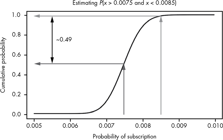{#fig-13-06fig-alt="Visually performing integration using the CDF"fig-align="center" width="70%"}#### Estimating Confidence Intervals> Looking at the probability of ranges of values leads us to a very> important concept in probability: the confidence interval. A> confidence interval is a lower and upper bound of values, typically> centered on the mean, describing a range of high probability, usually> 95, 99, or 99.9 percent. When we say something like "The 95 percent> confidence interval is from 12 to 20," what we mean is that there is a> 95 percent probability that our true measurement is somewhere between> 12 and 20. Confidence intervals provide a good method of describing> the range of possibilities when we're dealing with uncertain> information.In spite of a special note "*In Bayesian statistics what we are callinga "confidence interval" can go by a few other names, such as "criticalregion" or "critical interval." In some more traditional schools ofstatistics, "confidence interval" has a slightly different meaning,which is beyond the scope of this book.*" this concept and notions arenot correct for Bayesian statistics. At least what I have learnedreading other books, especially [@mcelreath2020].::: {.callout-warning}`r glossary("Bayesian statistics")` talks about `r glossary("credible interval", "credible intervals")` that have a very different meaning as the `r glossary("confidence interval", "confidence intervals")` of `r glossary("frequentist statistics")` McElreath even proposes the notion of `r glossary("compatibility interval", "compatibility intervals")`.:::> Say we wanted to know the range that covers 80 percent of the possible values for the true conversion rate. We solve this problem by combining our previous approaches: we draw lines at the y-axis from 0.1 and 0.9 to cover 80 percent, and then simply see where on the x-axis these intersect with our CDF: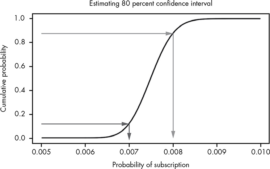{#fig-13-07fig-alt="Estimating our confidence intervals visually using the CDF"fig-align="center" width="70%"}### Using the CDF in R> Just as nearly all major PDFs have a function starting with $d$, like `dnorm()`, CDF functions start with $p$, such as `pnorm()`.::: {.callout-note}This is a new information for me. Now I understand better the differences and use cases of the different types of distribution. My comprehension will be fostered with the next section when the application of function starting with $q$ is explained.:::```{r}#| label: calc-beta-less-0.0065#| attr-source: '#lst-calc-beta-less-0.0065 lst-cap="Calculate the probability that Beta(300,39700) is less than 0.0065"'pbeta(0.0065,300,39700)``````{r}#| label: calc-beta-greater-0.0085#| attr-source: '#lst-calc-beta-greater-0.0085 lst-cap="Calculate the true probability that the conversion rate is greater than 0.0085"'pbeta(1,300,39700) -pbeta(0.0085,300,39700)```> The great thing about CDFs is that it doesn’t matter if your distribution is discrete or continuous. If we wanted to determine the probability of getting three or fewer heads in five coin tosses, for example, we would use the CDF for the binomial distribution like this:```{r}#| label: calc-beta-3-or-fewer-heads-5-tosses#| attr-source: '#lst-calc-beta-3-or-fewer-heads-5-tosses lst-cap="Calculate the probability of getting three or fewer heads in five coin tosses"'pbinom(3, 5, 0.5)```## The Quantile Function> Mathematically, the CDF is like any other function in that it takes an $x$ value, often representing the value we’re trying to estimate, and gives us a $y$ value, which represents the cumulative probability. But there is no obvious way to do this in reverse; that is, we can’t give the same function a $y$ to get an $x$.But we did reversing the function when we estimated the median in @sec-finding-the-median respectively in my version in @sec-replicate-figure-13-5.> The inverse of the CDF is an incredibly common and useful tool called the quantile function. To compute an exact value for our median and confidence interval, we need to use the quantile function for the beta distribution. ### Visualizing and Understanding the Quantile Function> Because the quantile function is simply the inverse of the CDF, it just looks like the CDF rotated 90 degrees, as shown in @fig-13-08.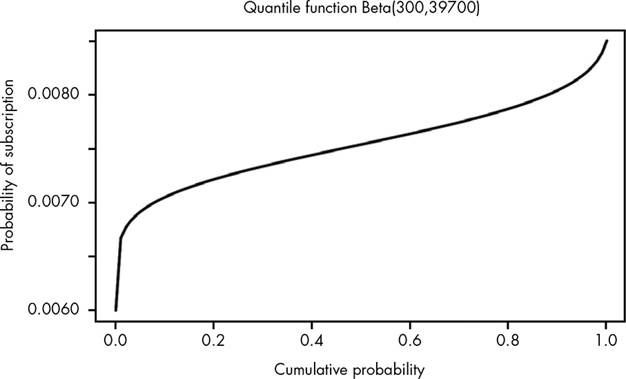{#fig-13-08fig-alt="Visually, the quantile function is just a rotation of the CDF"fig-align="center" width="70%"}> Whenever you hear phrases like:>> - “The top 10 percent of students …”> - “The bottom 20 percent of earners earn less than …”> - “The top quartile has notably better performance than …”>> you’re talking about values that are found using the quantile function### Calculating Quantiles in RWe are using the function `qnorm()` for calculating `r glossary("quantile", "quantiles")`.> For example, if we want to know the value that 99.9 percent of the distribution is less than, we can use qbeta() with the quantile we’re interested in calculating as the first argument, and the alpha and beta parameters of our beta distribution as the second and third arguments, like so:```{r}#| label: qbeta-less-99.9#| attr-source: '#lst-qbeta-less-99.9 lst-cap="Value that we 99.9 percent certain that the true conversion rate for our emails is less than 0.0089"' qbeta(0.999, 300, 39700)```The result is 0.0089, meaning we can be 99.9 percent certain that the true conversion rate for our emails is less than 0.0089.With the quantile function we can also calculate the 95% confidence interval by finding the lower and upper 2.5% quantile:```{r}#| label: get-95-conf-int#| attr-source: '#lst-get-95-conf-int lst-cap="Calculate the 95% confidence interval"'glue::glue("The lower bound is {round(qbeta(0.025,300,39700), 7)} and the upper bound is {round(qbeta(0.975,300,39700) ,7)}.")```> Now we can confidently say that we are 95 percent certain that the real conversion rate for blog visitors is somewhere between 0.67 percent and 0.84 percent. … Suppose an article on your blog goes viral and gets 100,000 visitors. Based on our calculations, we know that we should expect between 670 and 840 new email subscribers.## Wrapping Up## ExercisesTry answering the following questions to see how well you understand thetools of parameter estimation. The solutions can be found athttps://nostarch.com/learnbayes/.### Exercise 13-1Using the code example for plotting the PDF on page 127, plot the CDFand quantile functions.- For the CDF see @lst-fig-pb-13-4a and @fig-pb-13-4a.- For the quantile function see @lst-fig-pb-13-8 and @fig-pb-13-8.### Exercise 13-2Returning to the task of measuring snowfall from @sec-chap-10, say youhave the following measurements (in inches) of snowfall: 7.8, 9.4, 10.0,7.9, 9.4, 7.0, 7.0, 7.1, 8.9, 7.4What is your 99.9 percent confidence interval for the true value ofsnowfall?```{r}#| label: exr-13-2#| attr-source: '#lst-exr-13-2 lst-cap="Calculate the 99% confidence interval"'x <-c(7.8, 9.4, 10.0, 7.9, 9.4, 7.0, 7.0, 7.1, 8.9, 7.4)glue::glue("The lower bound is {round(qnorm(0.0005,mean(x), sd(x)), 2)} and the upper bound is {round(qnorm(0.9995,mean(x), sd(x)), 2)}.")```::: {.callout-warning}Besides that in my try I used the `sd_fun()` function from @lst-comp-sigma-with-own-function, I commit an error in using bounds of 0.001 and 0.999 instead of 0.0005 and 0.9995.:::### Exercise 13-3A child is going door to door selling candy bars. So far she has visited30 houses and sold 10 candy bars. She will visit 40 more houses today.What is the 95 percent confidence interval for how many candy bars shewill sell the rest of the day?```{r}#| label: exr-13-3#| attr-source: '#lst-exr-13-3 lst-cap="Calculate the 95 percent confidence interval for how many candy bars will be sold"'glue::glue("The lower bound is {round(qbeta(0.025, 10, 20), 2)}% and the upper bound is {round(qbeta(0.975, 10, 20), 2)}%.")glue::glue("This means that she will with 95% probability get between 40 * 0.18 = {40 * 0.18} and 40 * 0.51 = {40 * 0.51} candy bars.")glue::glue("But she can only sell complete bars: Therefore she will sell between {floor(40 * 0.18)} and {floor(40 * 0.51)} candy bars.")```## ExperimentsI started with @fig-pb-13-4a because this is the easiest graph, as itreplicates @fig-13-04 with just the CDF and nothing else. So maybe youwill begin also with this basic plot. After @fig-pb-13-4a the naturalsequence -- ordered by complexity -- is @fig-pb-13-3. After that you caninspect in detail my different tries with @fig-13-02 (@fig-pb-13-2a,@fig-pb-13-2b and my best solution @fig-pb-13-2c) . Then follow mysequences here from @fig-13-05 to @fig-13-08.::: callout-importantThere is the following system in using distributions with R, exemplifiedwith the normal distribution:- `dnorm` for plotting probability densities functions (PDFs).- `pnorm` for plotting cumulative distribution functions (CDFs).- `qnorm` for plotting quantile functions, it is the reverse of CDFs.- `rnorm` for generating and plotting random distributions.See1. R help file for [Distributions in the stats package](https://rdrr.io/r/stats/Distributions.html).2. [The distribution zoo](https://ben18785.shinyapps.io/distribution-zoo/) (a shiny application by [Ben Lambert](https://ben-lambert.com/bayesian/) & [Fergus Cooper](https://www.cs.ox.ac.uk/people/fergus.cooper/site/)). See for the code the [GitHub repo](https://github.com/ben18785/distribution-zoo).:::### Replicate Figure 13-1 {#sec-replicate-fig-13-1}#### Wrong dimension of x-axis for Figure 13-1At first I got the following graph:```{r}tibble::tibble(x =seq(0, 1, .0001),y =dbeta(x, 300, 39700)) |> ggplot2::ggplot(ggplot2::aes(x = x, y = y)) + ggplot2::geom_line()```The problem here is that the interesting part of the PDF is very smallas we know from the $\frac{300}{40000} = 0.0075$. Therefore it does notmake sense to spread the grid from 0 to 1. We get a much bettervisualization in the area 0 to 001:#### Better dimension of x-axis but still not identical for Figure 13-1```{r}tibble::tibble(x =seq(0, 0.01, .0001),y =dbeta(x, 300, 39700)) |> ggplot2::ggplot(ggplot2::aes(x = x, y = y)) + ggplot2::geom_line()```But even this curve is not optimal. Now let's try the interval \[0.005,0.01\]:#### Optimal dimension of x-axis but grid too wide for smooth Figure 13-1```{r}tibble::tibble(x =seq(0.005, 0.01, .0001),y =dbeta(x, 300, 39700)) |> ggplot2::ggplot(ggplot2::aes(x = x, y = y)) + ggplot2::geom_line()```It turns out that this is the interval also used in the book example.But in my visualization you can see some irregularity at the top,because my grid has too coarse. It has only 51 values. Let's try a muchfiner grid with 5001 values:#### Optimal replication of Figure 13-1```{r}tibble::tibble(x =seq(0.005, 0.01, .00001),y =dbeta(x, 300, 39700)) |> ggplot2::ggplot(ggplot2::aes(x = x, y = y)) + ggplot2::geom_line()```### Replicate Figure 13-2#### First try (bad)::: callout-noteI had to learn about the difference between `annotate(geom = "text" …)`and `annotate(geom = "label" …)`. There are two big differences:- `geom_text()` does not understand the `fill` aesthetics, e.g. you can't change the background color of the text.- `geom_label()` "is considerable slower than geom_text()" and does not support the `check_overlap` argument and the `angle` aesthetic. But more important for my use case `geom_label()` draws a rectangle around the label. You need to add `label.size = NA` to remove the label. Although the option `label.size` is documented ("Size of label border, in mm.") using `NA` to remove the border completely is not explained. I had to find out it the hard way via[StackOverflow](https://stackoverflow.com/a/58242703/7322615).:::```{r}#| label: fig-pb-13-2a#| fig-cap: "Visualizing the cumulative area under the curve"#| attr-source: '#lst-fig-pb-13-2a lst-cap="Highlighting the cumulative area under the curve"'#| out.width: 70%#| fig.align: centerx_lower <-seq(0.006, 0.0085, 0.0005)x_upper <-seq(0.0065, 0.009, 0.0005)text_pos <-seq(0.00625, 0.00875, 0.0005)colors <-c("gray90", "gray80", "gray70", "gray50", "gray40", "black") df_13_2 <-tibble::tibble(x =seq(0.006, 0.009, length.out =6000),y =dbeta(x, 300, 39700))ggplot2::ggplot(df_13_2, ggplot2::aes(x = x, y = y)) +ggplot2::geom_line() + ggplot2::geom_area(data = df_13_2 |> dplyr::filter(x >= x_lower[1] & x < x_upper[1]),fill = colors[1] ) + ggplot2::annotate(geom ="label", x = text_pos[1], size =5, y =125, color ="black", fill ="white", label.size =NA,label =round(integrate(function(x) dbeta(x, 300, 39700), x_lower[1], x_upper[1])[["value"]], 3)) + ggplot2::geom_area(data = df_13_2 |> dplyr::filter(x >= x_lower[2] & x < x_upper[2]),fill = colors[2] ) + ggplot2::annotate(geom ="label", x = text_pos[2], size =5, y =125, color ="black", fill ="white", label.size =NA,label =round(integrate(function(x) dbeta(x, 300, 39700), x_lower[1], x_upper[2])[["value"]], 3)) + ggplot2::geom_area(data = df_13_2 |> dplyr::filter(x >= x_lower[3] & x < x_upper[3]),fill = colors[3] ) + ggplot2::annotate(geom ="label", x = text_pos[3], size =5, y =125, color ="black", fill ="white", label.size =NA, label =round(integrate(function(x) dbeta(x, 300, 39700), x_lower[1], x_upper[3])[["value"]], 3)) + ggplot2::geom_area(data = df_13_2 |> dplyr::filter(x >= x_lower[4] & x < x_upper[4]),fill = colors[4] ) + ggplot2::annotate(geom ="label", x = text_pos[4], size =5, y =125, color ="black", fill ="white", label.size =NA, label =round(integrate(function(x) dbeta(x, 300, 39700), x_lower[1], x_upper[4])[["value"]], 3)) + ggplot2::geom_area(data = df_13_2 |> dplyr::filter(x >= x_lower[5] & x < x_upper[5]),fill = colors[5] ) + ggplot2::annotate("label", x = text_pos[5], size =5, y =125, color ="black", fill ="white", label.size =NA, label =round(integrate(function(x) dbeta(x, 300, 39700), x_lower[1], x_upper[5])[["value"]], 3)) + ggplot2::geom_area(data = df_13_2 |> dplyr::filter(x >= x_lower[6] & x < x_upper[6]),fill = colors[6] ) + ggplot2::annotate(geom ="label", x = text_pos[6], size =5, y =125, color ="black", fill ="white", label.size =NA, label =round(integrate(function(x) dbeta(x, 300, 39700), x_lower[1], x_upper[6])[["value"]], 3)) +ggplot2::theme_bw() +ggplot2::labs(title ="Visualizing the cumulative area under the curve",x ="Probability of Subscription",y ="Density")```#### Second try (Slightly better)::: callout-warningI am very unhappy about the many duplicates of @lst-fig-pb-13-2a. Itried to use loops or vectorized commands but the best I found out is@lst-fig-pb-13-2b with has still six duplicate code lines.:::```{r}#| label: fig-pb-13-2b#| fig-cap: "Visualizing the cumulative area under the curve"#| attr-source: '#lst-fig-pb-13-2b lst-cap="Highlighting the cumulative area under the curve"'#| out.width: 70%#| fig.align: centerx_lower <-seq(0.006, 0.0085, 0.0005)x_upper <-seq(0.0065, 0.009, 0.0005)label_x_pos <-seq(0.00625, 0.00875, 0.0005)colors <-c("gray90", "gray80", "gray70", "gray50", "gray40", "black") cum_rate =0for (i in1:6) { cum_rate[i] <-round(integrate(function(x) dbeta(x, 300, 39700), x_lower[1], x_upper[i])[["value"]], 3) }add_label <-function(x_pos, txt) { ggplot2::annotate(geom ="label",x = x_pos,y =125,size =5,label = txt,label.size =NA )}highlight_one_area <-function(df, i) { ggplot2::geom_area(data = df |> dplyr::filter(x >= x_lower[i] & x < x_upper[i]),fill = colors[i])}df_13_2 <- tibble::tibble(x =seq(0.006, 0.009, length.out =6000),y =dbeta(x, 300, 39700)) p_13_2 <- ggplot2::ggplot(df_13_2, ggplot2::aes(x = x, y = y)) + ggplot2::geom_line() +highlight_one_area(df_13_2, 1) +highlight_one_area(df_13_2, 2) +highlight_one_area(df_13_2, 3) +highlight_one_area(df_13_2, 4) +highlight_one_area(df_13_2, 5) +highlight_one_area(df_13_2, 6) +add_label(label_x_pos, cum_rate) + ggplot2::theme_bw() + ggplot2::labs(title ="Visualizing the cumulative area under the curve",x ="Probability of Subscription",y ="Density" )p_13_2```#### Third try (My best version)As I could not find a better solution for @lst-fig-pb-13-2b myself Iposted my question in[StackOverflow](https://stackoverflow.com/questions/77182234/ggplot2-shade-several-areas-under-the-curve-using-a-loop)and got an answer with two different options within one hour!The first solution is to use `lapply()`. I should have known that as Icame over a similar[solution](https://stackoverflow.com/a/18089991/7322615). The secondsolution is for me more complex and I have still to study it thoroughlyto understand it.What follows in @lst-fig-pb-13-2c is the modern take of `lapply()` usingthe `purrr::map()` function. (I do not understand why I had to useexactly the argument "df" and asked via SO comment.)```{r}#| label: fig-pb-13-2c#| fig-cap: "Visualizing the cumulative area under the curve"#| attr-source: '#lst-fig-pb-13-2c lst-cap="Highlighting the cumulative area under the curve"'#| out.width: 70%#| fig.align: center########### Vectors ##############x_lower <-seq(0.006, 0.0085, 0.0005)x_upper <-seq(0.0065, 0.009, 0.0005)label_x_pos <-seq(0.00625, 0.00875, 0.0005)colors <-c("gray90", "gray80", "gray70", "gray50", "gray40", "black") ########### Functions ############cum_rate =0for (i in1:6) { cum_rate[i] <-round(integrate(function(x) dbeta(x, 300, 39700), x_lower[1], x_upper[i])[["value"]], 3) }add_label <-function(x_pos, txt) { ggplot2::annotate(geom ="label",x = x_pos,y =125,size =5,label = txt,label.size =NA )}highlight_areas <-function(df, i) { ggplot2::geom_area(data = df |> dplyr::filter(x >= x_lower[i] & x < x_upper[i]),fill = colors[i])}######### Graph plotting ############df_13_2 <- tibble::tibble(x =seq(0.006, 0.009, length.out =6000),y =dbeta(x, 300, 39700)) p_13_2 <- ggplot2::ggplot(df_13_2, ggplot2::aes(x = x, y = y)) + ggplot2::geom_line() + purrr::map(1:6, highlight_areas, df = df_13_2) +add_label(label_x_pos, cum_rate) + ggplot2::theme_bw() + ggplot2::labs(title ="Visualizing the cumulative area under the curve",x ="Probability of Subscription",y ="Density" )p_13_2```### Replicate Figure 13-3```{r}#| label: fig-pb-13-3#| fig-cap: "Plotting just the cumulative probability from Figure 13-2"#| attr-source: '#lst-fig-pb-13-3 lst-cap="Plot the cumulative area under the curve"'#| out.width: 70%#| fig.align: centerdf_13_3 <-tibble::tibble(x =seq(0.006, 0.009, 0.0005),y =pbeta(x, 300, 39700)) ggplot2::ggplot(df_13_3, ggplot2::aes(x = x, y = y)) + ggplot2::geom_point() + ggplot2::theme_bw() + ggplot2::labs(title ="The cumulative distribution function",x ="Subscription rate",y ="Cumulative Probability" )```### Replicate Figure 13-4#### Cumulative Distribution Function (CDF)```{r}#| label: fig-pb-13-4a#| fig-cap: "The CDF for our problem"#| attr-source: '#lst-fig-pb-13-4a lst-cap="Plot the Cumulative Distribution Function (CDF)"'#| out.width: 70%#| fig.align: centerdf_13_4a <-tibble::tibble(x =seq(0.005, 0.01, 1e-6),y =pbeta(x, 300, 39700)) ggplot2::ggplot(df_13_4a, ggplot2::aes(x = x, y = y)) + ggplot2::geom_line() + ggplot2::theme_bw() + ggplot2::labs(title ="The cumulative distribution function",x ="Subscription rate",y ="Cumulative Probability" )```#### Empiricial Cumulative Distribution Function (ECDF) - with steps::: callout-noteTrying to apply the CDF I noticed that there is also an`r`glossary("ECDF")\` (Empirical Cumulative Distribution Function). Thedifferences are that the ECDF is a step function whereas the CDF issmooth. But with many different values the ECDF approximates to tasmooth function.:::```{r}#| label: fig-pb-13-4b#| fig-cap: "The ECDF for our problem"#| attr-source: '#lst-fig-pb-13-4b lst-cap="Plot the Empirical Cumulative Distribution Function (ECDF)"'#| out.width: 70%#| fig.align: centerdf_13_4b <-tibble::tibble(x =seq(0.005, 0.01, 1e-4),y =rbeta(x, 300, 39700)) ggplot2::ggplot(df_13_4b, ggplot2::aes(y)) + ggplot2::stat_ecdf(geom ="step") + ggplot2::theme_bw() + ggplot2::labs(title ="The empirical cumulative distribution function (ECDF)",x ="x",y ="ECDF" )```#### Empiricial Cumulative Distribution Function (ECDF) - with points```{r}#| label: fig-pb-13-4c#| fig-cap: "The ECDF for our problem"#| attr-source: '#lst-fig-pb-13-4c lst-cap="Plot the Cumulative Distribution Function (CDF)"'#| out.width: 70%#| fig.align: centerdf_13_4c <-tibble::tibble(x =seq(0.005, 0.01, 1e-4),y =rbeta(x, 300, 39700)) ggplot2::ggplot(df_13_4c, ggplot2::aes(y)) + ggplot2::stat_ecdf(geom ="point") + ggplot2::theme_bw() + ggplot2::labs(title ="The empirical cumulative distribution function (ECDF)",x ="x",y ="ECDF" )```#### Empiricial Cumulative Distribution Function (ECDF) - smooth```{r}#| label: fig-pb-13-4d#| fig-cap: "The ECDF for our problem"#| attr-source: '#lst-fig-pb-13-4d lst-cap="Plot the Empirical Cumulative Distribution Function (ECDF)"'#| out.width: 70%#| fig.align: centerdf_13_4d <-tibble::tibble(x =seq(0.005, 0.01, 1e-6),y =rbeta(x, 300, 39700)) ggplot2::ggplot(df_13_4d, ggplot2::aes(y)) + ggplot2::stat_ecdf(geom ="step") + ggplot2::theme_bw() + ggplot2::labs(title ="The empirical cumulative distribution function (ECDF)",x ="x",y ="ECDF" )```### Replicate Figure 13-5 {#sec-replicate-figure-13-5}```{r}#| label: fig-pb-13-5#| fig-cap: "Estimating the median visually using the CDF"#| attr-source: '#lst-fig-pb-15 lst-cap="Estimate and display median using the CDF"'#| out.width: 70%#| fig.align: centermedian_beta <-round(qbeta(0.5, 300, 39700), 5)df_13_5 <-tibble::tibble(x =seq(0.005, 0.01, 1e-6),y =pbeta(x, 300, 39700)) ggplot2::ggplot(df_13_5, ggplot2::aes(x = x, y = y)) + ggplot2::geom_line() + ggplot2::geom_segment(ggplot2::aes(x =0.005, y =0.50, xend = median_beta, yend =0.50),lineend ="square", linejoin ="bevel", color ="steelblue",size =0.8, arrow = ggplot2::arrow(length = ggplot2::unit(0.5, "cm"))) + ggplot2::geom_segment(ggplot2::aes(x = median_beta, y =0.50, xend = median_beta, yend =0.00),lineend ="square", linejoin ="bevel", color ="steelblue",size =0.8, arrow = ggplot2::arrow(length = ggplot2::unit(0.5, "cm"))) + ggplot2::annotate("text", y =0.625, x =0.0087,label ="median = qbeta(0.5, 300, 39700)") + ggplot2::annotate("text", y =0.55, x =0.0087,label = glue::glue("= {median_beta}")) + ggplot2::theme_bw() + ggplot2::labs(title ="Estimating median",x ="Probability of subscription",y ="Cumulative Probability" )```### Replicate Figure 13-6 {#sec-replicate-figure-13-6}In contrast to @fig-pb-13-5 where I cheated by calculating the median ofthe beta distribution I will in @sec-replicate-figure-13-6 try to approximate theintegration just visually.We are going to estimate the range between p(x \> 0.0075 and x \<0.0085). The solution could be visually done approximately either with aruler or (not so exact) just by eyeballing. To do it programmaticallywithout integration is a somewhat complex procedure with four steps:1. First I have to draw vertical lines from the start and end of the interesting range. These lines have to cross the CDF because I do not know the value of the cumulative probability where they meet the CDF.2. Then I have to inspect the intersection visually and try to estimate and draw the horizontal lines. This has to be done several times until the two lines cross (almost) exactly at the CDF.3. Now I can limit the vertical and horizontal lines, so that they stop at the CDF.4. The last step is to estimate the range by reading the intersection at the y-axis.#### First step```{r}#| label: fig-pb-13-6a#| fig-cap: "Visually performing integration using the CDF: First step"#| attr-source: '#lst-fig-pb-13-6a lst-cap="Approximate the integration of a range of the CDF: First step"'#| out.width: 70%#| fig.align: centerdf_13_6 <-tibble::tibble(x =seq(0.005, 0.01, 1e-6),y =pbeta(x, 300, 39700)) ggplot2::ggplot(df_13_6, ggplot2::aes(x = x, y = y)) + ggplot2::geom_line() + ggplot2::geom_vline(xintercept =0.0075, color ="steelblue",linetype ="dashed") + ggplot2::geom_vline(xintercept =0.0085, color ="steelblue",linetype ="dashed") + ggplot2::theme_bw() + ggplot2::labs(title ="Estimating P(x > 0.0075 and x < 0.0085)",x ="Probability of subscription",y ="Cumulative Probability" )```#### Second stepThe lower cumulative probability is almost exact 0.5 as I can see andalready know from @fig-pb-13-5. Without knowing the solution in the bookmy first approach was to draw a line at 0.98% of the CDF (orange). Asthis seems a little to less a tried with it .99%```{r}#| label: fig-pb-13-6b#| fig-cap: "Visually performing integration using the CDF: Second step"#| attr-source: '#lst-fig-pb-13-6b lst-cap="Approximate the integration of a range of the CDF: Second step"'#| out.width: 70%#| fig.align: centerdf_13_6 <-tibble::tibble(x =seq(0.005, 0.01, 1e-6),y =pbeta(x, 300, 39700)) ggplot2::ggplot(df_13_6, ggplot2::aes(x = x, y = y)) + ggplot2::geom_line() + ggplot2::geom_vline(xintercept =0.0075, color ="steelblue",linetype ="dashed") + ggplot2::geom_vline(xintercept =0.0085, color ="steelblue",linetype ="dashed") + ggplot2::geom_hline(yintercept =0.5, color ="steelblue",linetype ="dashed") + ggplot2::geom_hline(yintercept =0.98, color ="orange",linetype ="dashed") + ggplot2::geom_hline(yintercept =0.99, color ="steelblue",linetype ="dashed") + ggplot2::theme_bw() + ggplot2::labs(title ="Estimating P(x > 0.0075 and x < 0.0085)",x ="Probability of subscription",y ="Cumulative Probability" )```#### Third step```{r}#| label: fig-pb-13-6c#| fig-cap: "Visually performing integration using the CDF: Third step"#| attr-source: '#lst-fig-pb-13-6c lst-cap="Approximate the integration of a range of the CDF: Third step"'#| out.width: 70%#| fig.align: centerdf_13_6 <-tibble::tibble(x =seq(0.005, 0.01, 1e-6),y =pbeta(x, 300, 39700)) ggplot2::ggplot(df_13_6, ggplot2::aes(x = x, y = y)) + ggplot2::geom_line() + ggplot2::geom_segment( ggplot2::aes(xend =0.005, yend =0.50, x =0.00750, y =0.50),lineend ="square", linejoin ="bevel", color ="steelblue",size =0.8, arrow = ggplot2::arrow(length = ggplot2::unit(0.5, "cm"))) + ggplot2::geom_segment( ggplot2::aes(xend =0.0075, yend =0.50, x =0.0075, y =0.00),lineend ="square", linejoin ="bevel", color ="steelblue",size =0.8, arrow = ggplot2::arrow(length = ggplot2::unit(0.5, "cm"))) + ggplot2::geom_segment( ggplot2::aes(x =0.0085, y =0,xend =0.0085, yend =0.99),lineend ="square", linejoin ="bevel", color ="steelblue",size =0.8, arrow = ggplot2::arrow(length = ggplot2::unit(0.5, "cm"))) + ggplot2::geom_segment( ggplot2::aes(x =0.0085, y =0.99,xend =0.005, yend =0.99),lineend ="square", linejoin ="bevel", color ="steelblue",size =0.8, arrow = ggplot2::arrow(length = ggplot2::unit(0.5, "cm"))) + ggplot2::theme_bw() + ggplot2::labs(title ="Estimating P(x > 0.0075 and x < 0.0085)",x ="Probability of subscription",y ="Cumulative Probability" )```#### Fourth step```{r}#| label: fig-pb-13-6d#| fig-cap: "Visually performing integration using the CDF: Fourth step"#| attr-source: '#lst-fig-pb-13-6d lst-cap="Approximate the integration of a range of the CDF: Fourth step"'#| out.width: 70%#| fig.align: centerdf_13_6 <-tibble::tibble(x =seq(0.005, 0.01, 1e-6),y =pbeta(x, 300, 39700)) ggplot2::ggplot(df_13_6, ggplot2::aes(x = x, y = y)) + ggplot2::geom_line() + ggplot2::geom_segment( ggplot2::aes(xend =0.005, yend =0.50, x =0.00750, y =0.50),lineend ="square", linejoin ="bevel", color ="steelblue",size =0.8, arrow = ggplot2::arrow(length = ggplot2::unit(0.5, "cm"))) + ggplot2::geom_segment( ggplot2::aes(xend =0.0075, yend =0.50, x =0.0075, y =0.00),lineend ="square", linejoin ="bevel", color ="steelblue",size =0.8, arrow = ggplot2::arrow(length = ggplot2::unit(0.5, "cm"))) + ggplot2::geom_segment( ggplot2::aes(x =0.0085, y =0,xend =0.0085, yend =0.99),lineend ="square", linejoin ="bevel", color ="steelblue",size =0.8, arrow = ggplot2::arrow(length = ggplot2::unit(0.5, "cm"))) + ggplot2::geom_segment( ggplot2::aes(x =0.0085, y =0.99,xend =0.005, yend =0.99),lineend ="square", linejoin ="bevel", color ="steelblue",size =0.8, arrow = ggplot2::arrow(length = ggplot2::unit(0.5, "cm"))) + ggplot2::geom_segment( ggplot2::aes(x =0.0055, y =0.5,xend =0.0055, yend =0.99),lineend ="square", linejoin ="bevel", color ="red",size =0.8, arrow = ggplot2::arrow(length = ggplot2::unit(0.5, "cm"))) + ggplot2::geom_segment( ggplot2::aes(xend =0.0055, yend =0.5,x =0.0055, y =0.99),lineend ="square", linejoin ="bevel", color ="red",size =0.8, arrow = ggplot2::arrow(length = ggplot2::unit(0.5, "cm"))) + ggplot2::annotate("text", x =0.0058, y =0.75,label ="~ 0.49", color ="red", size =5) + ggplot2::theme_bw() + ggplot2::labs(title ="Estimating P(x > 0.0075 and x < 0.0085)",x ="Probability of subscription",y ="Cumulative Probability" )```### Replicate Figure 13-7There is nothing new for approximating the range that covers 80 percent of the possible values for the true conversion rate. We use the same strategy as in @sec-replicate-figure-13-6 but this time starting from the y-axis:```{r}#| label: fig-pb-13-7#| fig-cap: "Estimating our confidence intervals visually using the CDF"#| attr-source: '#lst-fig-pb-13-7 lst-cap="Approximate the confidence interval via the CDF"'#| out.width: 70%#| fig.align: centerdf_13_7 <-tibble::tibble(x =seq(0.005, 0.01, 1e-6),y =pbeta(x, 300, 39700)) ggplot2::ggplot(df_13_7, ggplot2::aes(x = x, y = y)) + ggplot2::geom_line() + ggplot2::geom_segment( ggplot2::aes(xend =0.007, yend =0.125, x =0.005, y =0.125),lineend ="square", linejoin ="bevel", color ="steelblue",size =0.6, arrow = ggplot2::arrow(length = ggplot2::unit(0.5, "cm"))) + ggplot2::geom_segment( ggplot2::aes(xend =0.0080, yend =0.875, x =0.005, y =0.875),lineend ="square", linejoin ="bevel", color ="steelblue",size =0.6, arrow = ggplot2::arrow(length = ggplot2::unit(0.5, "cm"))) + ggplot2::geom_segment( ggplot2::aes(x =0.007, y =0.125,xend =0.007, yend =0.0),lineend ="square", linejoin ="bevel", color ="steelblue",size =0.6, arrow = ggplot2::arrow(length = ggplot2::unit(0.5, "cm"))) + ggplot2::geom_segment( ggplot2::aes(x =0.008, y =0.875,xend =0.008, yend =0.0),lineend ="square", linejoin ="bevel", color ="steelblue",size =0.6, arrow = ggplot2::arrow(length = ggplot2::unit(0.5, "cm"))) + ggplot2::theme_bw() + ggplot2::labs(title ="Estimating 80% Confidence Interval",x ="Probability of subscription",y ="Cumulative Probability" )```### Replicate Figure 13-8```{r}#| label: fig-pb-13-8#| fig-cap: "Visually, the quantile function is just a rotation of the CDF."#| attr-source: '#lst-fig-pb-13-8 lst-cap="Plot the quantile function"'#| out.width: 70%#| fig.align: centerdf_13_8 <-tibble::tibble(x =seq(0, 1, 1e-4),y =qbeta(x, 300, 39700)) ggplot2::ggplot(df_13_8, ggplot2::aes(x = x, y = y)) + ggplot2::ylim(0.006, 0.009) + ggplot2::geom_line() + ggplot2::theme_bw() + ggplot2::labs(title ="Quantile Function Beta(300, 39700)",x ="Subscription rate",y ="Cumulative Probability" )```