Chapter 3 Preparation des donnees H2

### Charger les bibliothèques ###
library(ade4)
library(amt)
library(ape)
library(car)
library(data.table)
library(dplyr)
library(gclus)
library(ggplot2)
library(ggpmisc)
library(ggpubr)
library(gridExtra)
library(janitor)
library(lubridate)
library(mapview)
library(pals)
library(performance)
library(readxl)
library(SciViews)
library(sf)
library(tidyverse)
library(vegan)
options(ggrepel.max.overlaps = Inf)
options(scipen=999)

setwd("C:/Users/Sarah/Desktop/Maitrise/Données/")

3.1 Aires d’études par région

Le but de cette section est de créer une polygone de chaque aire d’étude en réalisant un MCP 100% sur tous les points d’un secteur/année.

######## 1. Aires d'études par région ########

# Charger les données
locs8 = readRDS("C:/Users/Sarah/Desktop/Maitrise/Données/Data/locs8.rds")
data_fem <- readRDS(file = "C:/Users/Sarah/Desktop/Maitrise/Données/Data/data_hyp1_final.rds")

# Vérifier le CRS des points
st_crs(locs8) # 32198

## Coordinate Reference System:
##   User input: EPSG:32198 
##   wkt:
## PROJCRS["NAD83 / Quebec Lambert",
##     BASEGEOGCRS["NAD83",
##         DATUM["North American Datum 1983",
##             ELLIPSOID["GRS 1980",6378137,298.257222101,
##                 LENGTHUNIT["metre",1]]],
##         PRIMEM["Greenwich",0,
##             ANGLEUNIT["degree",0.0174532925199433]],
##         ID["EPSG",4269]],
##     CONVERSION["Quebec Lambert Projection",
##         METHOD["Lambert Conic Conformal (2SP)",
##             ID["EPSG",9802]],
##         PARAMETER["Latitude of false origin",44,
##             ANGLEUNIT["degree",0.0174532925199433],
##             ID["EPSG",8821]],
##         PARAMETER["Longitude of false origin",-68.5,
##             ANGLEUNIT["degree",0.0174532925199433],
##             ID["EPSG",8822]],
##         PARAMETER["Latitude of 1st standard parallel",60,
##             ANGLEUNIT["degree",0.0174532925199433],
##             ID["EPSG",8823]],
##         PARAMETER["Latitude of 2nd standard parallel",46,
##             ANGLEUNIT["degree",0.0174532925199433],
##             ID["EPSG",8824]],
##         PARAMETER["Easting at false origin",0,
##             LENGTHUNIT["metre",1],
##             ID["EPSG",8826]],
##         PARAMETER["Northing at false origin",0,
##             LENGTHUNIT["metre",1],
##             ID["EPSG",8827]]],
##     CS[Cartesian,2],
##         AXIS["easting (X)",east,
##             ORDER[1],
##             LENGTHUNIT["metre",1]],
##         AXIS["northing (Y)",north,
##             ORDER[2],
##             LENGTHUNIT["metre",1]],
##     USAGE[
##         SCOPE["Topographic mapping (medium and small scale)."],
##         AREA["Canada - Quebec."],
##         BBOX[44.99,-79.85,62.62,-57.1]],
##     ID["EPSG",32198]]

locs8 %>% dplyr::select(long_proj, lat_proj) %>% head() # ok

## Simple feature collection with 6 features and 2 fields
## Geometry type: POINT
## Dimension:     XY
## Bounding box:  xmin: -379255 ymin: 394616.8 xmax: -377263.9 ymax: 395095
## Projected CRS: NAD83 / Quebec Lambert
##       long_proj lat_proj                   geometry
## 1...1 -378650.8 394721.7 POINT (-378650.8 394721.7)
## 2...2 -378699.9 394773.4 POINT (-378699.9 394773.4)
## 3...3 -379255.0 394765.7   POINT (-379255 394765.7)
## 4...4 -377263.9 395095.0   POINT (-377263.9 395095)
## 5...5 -379192.0 394733.8   POINT (-379192 394733.8)
## 6...6 -379172.1 394616.8 POINT (-379172.1 394616.8)

# Nb individus
length(unique(locs8$ID_Animal_Annee)) # 258

## [1] 258

# Faire les tracks (un par site)
tracks_dv <- make_track(locs8, long_proj, lat_proj, Date_Heure_QC, Site, crs = 32198)

# Faire le MCP 100% par site
mcp_dv <- tracks_dv %>%
  nest(data = -Site) %>%
  mutate(mcp = map(data, ~ hr_mcp(., levels = 1)), n = map_int(data, nrow)) %>%
  hr_to_sf(mcp, Site, n)

st_crs(mcp_dv) # Ok, encore en 32198

## Coordinate Reference System:
##   User input: EPSG:32198 
##   wkt:
## PROJCRS["NAD83 / Quebec Lambert",
##     BASEGEOGCRS["NAD83",
##         DATUM["North American Datum 1983",
##             ELLIPSOID["GRS 1980",6378137,298.257222101,
##                 LENGTHUNIT["metre",1]]],
##         PRIMEM["Greenwich",0,
##             ANGLEUNIT["degree",0.0174532925199433]],
##         ID["EPSG",4269]],
##     CONVERSION["Quebec Lambert Projection",
##         METHOD["Lambert Conic Conformal (2SP)",
##             ID["EPSG",9802]],
##         PARAMETER["Latitude of false origin",44,
##             ANGLEUNIT["degree",0.0174532925199433],
##             ID["EPSG",8821]],
##         PARAMETER["Longitude of false origin",-68.5,
##             ANGLEUNIT["degree",0.0174532925199433],
##             ID["EPSG",8822]],
##         PARAMETER["Latitude of 1st standard parallel",60,
##             ANGLEUNIT["degree",0.0174532925199433],
##             ID["EPSG",8823]],
##         PARAMETER["Latitude of 2nd standard parallel",46,
##             ANGLEUNIT["degree",0.0174532925199433],
##             ID["EPSG",8824]],
##         PARAMETER["Easting at false origin",0,
##             LENGTHUNIT["metre",1],
##             ID["EPSG",8826]],
##         PARAMETER["Northing at false origin",0,
##             LENGTHUNIT["metre",1],
##             ID["EPSG",8827]]],
##     CS[Cartesian,2],
##         AXIS["easting (X)",east,
##             ORDER[1],
##             LENGTHUNIT["metre",1]],
##         AXIS["northing (Y)",north,
##             ORDER[2],
##             LENGTHUNIT["metre",1]],
##     USAGE[
##         SCOPE["Topographic mapping (medium and small scale)."],
##         AREA["Canada - Quebec."],
##         BBOX[44.99,-79.85,62.62,-57.1]],
##     ID["EPSG",32198]]

# Admirer le résultat
mapview(mcp_dv) # ok!

# Vérifier avec les points
library(rnaturalearth)
library(rnaturalearthdata) # Car mapview bugge

## 
## Attachement du package : 'rnaturalearthdata'

## L'objet suivant est masqué depuis 'package:rnaturalearth':
## 
##     countries110

canada <- ne_countries(country = "canada") 

# Subset des points
pts_verif = locs8 %>%
  sample_n(nrow(locs8)/10) # 10%

ggplot(data = canada) +
  geom_sf() +
  geom_sf(data = mcp_dv, fill = "lightblue") + 
  geom_sf(data = pts_verif, size = 2, shape = 21, fill = "darkred") + 
  coord_sf(xlim = c(-78, -64), ylim = c(51, 45), expand = FALSE)

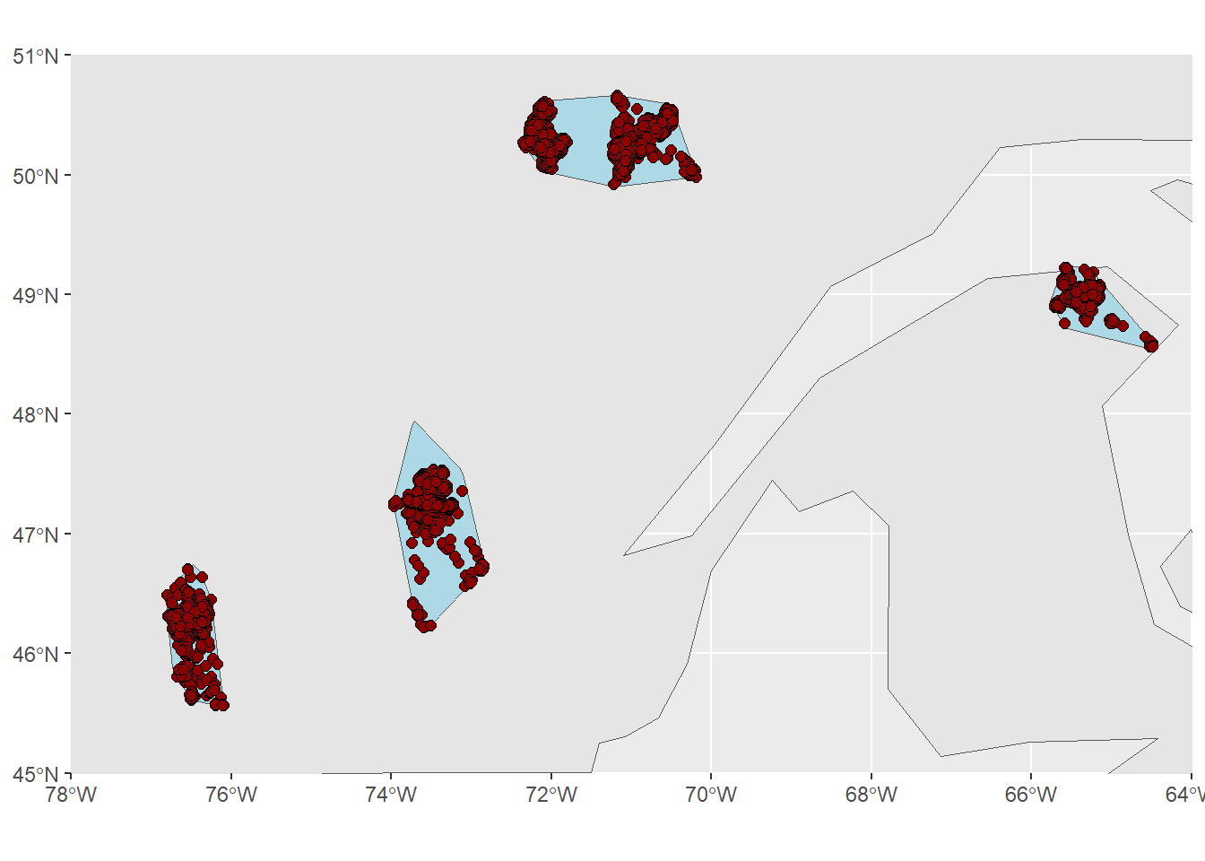
# Ajouter un buffer au tour
# 95% : 0.575km de distance par heure, donc *3 arrondi on va mettre 2km pour être sûrs.

mcp_dv # Units = mètres

## Simple feature collection with 4 features and 5 fields
## Geometry type: POLYGON
## Dimension:     XY
## Bounding box:  xmin: -637960.1 ymin: 205917.9 xmax: 294746.7 ymax: 742987.8
## Projected CRS: NAD83 / Quebec Lambert
##   level     what              area      Site      n
## 1     1 estimate 10137703532 [m^2]  Mauricie 115429
## 2     1 estimate 10015382589 [m^2]      SLSJ 108551
## 3     1 estimate  4897277832 [m^2] Outaouais  74605
## 4     1 estimate  3685249817 [m^2]  Gaspesie  11869
##                         geometry
## 1 POLYGON ((-330473.9 314992....
## 2 POLYGON ((-121304.3 671323....
## 3 POLYGON ((-592742.1 206783,...
## 4 POLYGON ((292080 521330.8, ...

mcp_dv2 = st_buffer(mcp_dv, 2000)
mapview(mcp_dv) + mapview(mcp_dv2) # ok!

# Sauvegarder mcp_dv2
#saveRDS(mcp_dv2, "Data/mcp_dv2.rds")

3.2 Intersection avec les cartes

Ensuite, je fais l’intersection entre l’aire d’étude calculée à la section précédente et la carte écoforestière correspondante pour chaque secteur/année. Puisque c’est le même principe qui se répète, j’ai mis seulement Mauricie 2015 en example.

# Charger les données
scores_hab <- readRDS("C:/Users/Sarah/Desktop/Maitrise/Données/Data/scores_nourriture_final.rds")
mcp_dv2 <- readRDS("C:/Users/Sarah/Desktop/Maitrise/Données/Data/mcp_dv2.rds")
locs8 <- readRDS("C:/Users/Sarah/Desktop/Maitrise/Données/Data/locs8.rds")

mcp_Mauricie = mcp_dv2[1,]
mcp_SLSJ = mcp_dv2[2,]
mcp_Outaouais = mcp_dv2[3,]
mcp_Gaspesie = mcp_dv2[4,]

# Créer les catégories Eau et Agricole dans HABOURS
coter_eau <- c("EAU", "ILE", "INO")
coter_agri <- c("A", "AF")
coter_anthro <- c("ANT", "NF", "GR", "RO", "CFO","AEP", "DEP")


#### 2015: Locs Mauricie ####

locs8 %>% as.data.frame %>%
  filter(Annee == "2015") %>%
  group_by(Site) %>%
  summarise(n = n()) # Mauricie

## # A tibble: 1 × 2
##   Site         n
##   <fct>    <int>
## 1 Mauricie 13046

 # Charger la carte
 carte_2015 <- sf::st_read("C:/Users/Sarah/Desktop/Maitrise/Données/Data/Ours_noir_mai_2022/Peup_Ecofor_Sites_Etude_Ours_2016_2020_new.gdb",
                           layer = "Peupl_Eco_mauricie_2016")

## Reading layer `Peupl_Eco_mauricie_2016' from data source 
##   `C:\Users\sarah\Desktop\Maitrise\Données\Data\Ours_noir_mai_2022\Peup_Ecofor_Sites_Etude_Ours_2016_2020_new.gdb' 
##   using driver `OpenFileGDB'

## Warning in CPL_read_ogr(dsn, layer, query, as.character(options), quiet, : GDAL
## Message 1: organizePolygons() received a polygon with more than 100 parts. The
## processing may be really slow.  You can skip the processing by setting
## METHOD=SKIP, or only make it analyze counter-clock wise parts by setting
## METHOD=ONLY_CCW if you can assume that the outline of holes is counter-clock
## wise defined

## Simple feature collection with 471679 features and 97 fields
## Geometry type: MULTIPOLYGON
## Dimension:     XY
## Bounding box:  xmin: -458007.4 ymin: 250841.2 xmax: -320488.3 ymax: 489989.8
## Projected CRS: NAD83 / Quebec Lambert

 # Corriger le nom des habitats
 carte_2015$HABOURS <- recode_factor(carte_2015$HABOURS,
                                 "Coupe_05" = "C_0-5", #1
                                 "Coupe_610" = "C_6-10", #2
                                 "Brulis_020" = "BR_0-20", #3
                                 "Coupe_1120" = "C_11-20", #4
                                 "M_50+" = "M_50", #5
                                 "M_30" = "M_30", #6
                                 "F_30" = "F_30", #7
                                 "F_50+" = "F_50", #8
                                "PES_30" = "PES_30", #9
                                 "DS_DH" = "DS-DH", #10
                                 "PES_50+" = "PES_50", #11
                                 "SAP_30" = "SAP_30", #12
                                 "SAP_50+" = "SAP_50",
                                 "EAU" = "Eau") %>% #13
   droplevels()

 # Créer l'intersection entre les MCP et la carte
 inter_2015 <- st_intersection(mcp_Mauricie, carte_2015)

## Warning: attribute variables are assumed to be spatially constant throughout
## all geometries

 # Vérifier le résultat avec une fraction des données
 mapview(sample_n(inter_2015, nrow(inter_2015)/100))

 # Créer colonne superficie en m2
 inter_2015$area_m2 = st_area(inter_2015)

 # Répartition des habitats
 sup_2015 = inter_2015 %>% as.data.frame() %>%
   group_by(Habitat = as.factor(HABOURS)) %>% # Colonne habitat
   summarise(Site = as.factor("Mauricie"),  # Colonne site
             Superficie_m2 = sum(area_m2)) %>% # Superficie totale par habitat
   mutate(Pourcentage = as.numeric(Superficie_m2/sum(Superficie_m2)*100)) # Proportion

head(sup_2015)

## # A tibble: 6 × 4
##   Habitat Site     Superficie_m2 Pourcentage
##   <fct>   <fct>            [m^2]       <dbl>
## 1 C_0-5   Mauricie    326654873.        2.96
## 2 C_6-10  Mauricie    332159711.        3.01
## 3 BR_0-20 Mauricie    119346530.        1.08
## 4 C_11-20 Mauricie   1349961891.       12.2 
## 5 M_50    Mauricie   3135662855.       28.4 
## 6 M_30    Mauricie    455898231.        4.14

 # Vérifications
 str(sup_2015) # ok

## tibble [17 × 4] (S3: tbl_df/tbl/data.frame)
##  $ Habitat      : Factor w/ 17 levels "C_0-5","C_6-10",..: 1 2 3 4 5 6 7 8 9 10 ...
##  $ Site         : Factor w/ 1 level "Mauricie": 1 1 1 1 1 1 1 1 1 1 ...
##  $ Superficie_m2: Units: [m^2] num [1:17] 326654873 332159711 119346530 1349961891 3135662855 ...
##  $ Pourcentage  : num [1:17] 2.96 3.01 1.08 12.25 28.45 ...

 sum(sup_2015$Pourcentage) # 100: ok

## [1] 100

 st_area(mcp_dv2) # 11 023 294 601

## Units: [m^2]
## [1] 11023294601 10820363115  5528527514  4226072945

 sum(sup_2015$Superficie_m2) # 11 023 294 601 = ok

## 11023294601 [m^2]

Cela nous donne la proportion de chaque habitat (total: 100%) dans tous les secteurs/année. Il faut alors lier le Site-Habitat-Année avec les scores correspondants. Puis, je calcule le score * proportion d’habitat dans le secteur. Ces blocs, qui totalisent 100%, seront additionnés plus tard pour créer la moyenne pondérée du score. J’ai choisi de ne pas diviser par 100 le pourcentage pour éviter de travailler avec de minuscules nombres

# # Lier avec les scores d'habitat
 scores_2015 = scores_hab %>%
   filter(Annee == "2015") %>%
   merge(x = ., y = sup_2015, by = c("Site", "Habitat"), all.y = TRUE) %>%
   mutate(Score_Graminees_Pond = Score_Graminees*Pourcentage,
          Score_Fruits_Pond = Score_Fruits*Pourcentage,
          Score_Fourmis_Pond = Score_Fourmis*Pourcentage,
          Score_Noix_Pond = Score_Noix*Pourcentage)

# Sauvegarder le résultat
#saveRDS(scores_2015, "Data/h2_scores2015.rds")

3.3 Tout mettre ensemble

Il faut lier les scores des habitats avec les données des femelles. Je commence par charger toutes les données de scores.

#### 3. Tout mettre ensemble ####
data_fem <- readRDS(file = "C:/Users/Sarah/Desktop/Maitrise/Données/Data/data_hyp1_final.rds")

scores_2015 = readRDS("C:/Users/Sarah/Desktop/Maitrise/Données/Data/h2_scores2015.rds")
scores_2016 = readRDS("C:/Users/Sarah/Desktop/Maitrise/Données/Data/h2_scores2016.rds")
scores_2017 = readRDS("C:/Users/Sarah/Desktop/Maitrise/Données/Data/h2_scores2017.rds")
scores_2018 = readRDS("C:/Users/Sarah/Desktop/Maitrise/Données/Data/h2_scores2018.rds")
scores_2019 = readRDS("C:/Users/Sarah/Desktop/Maitrise/Données/Data/h2_scores2019.rds")
scores_2020 = readRDS("C:/Users/Sarah/Desktop/Maitrise/Données/Data/h2_scores2020.rds")
scores_2021 = readRDS("C:/Users/Sarah/Desktop/Maitrise/Données/Data/h2_scores2021.rds")
scores_2022 = readRDS("C:/Users/Sarah/Desktop/Maitrise/Données/Data/h2_scores2022.rds")

scores_complet = rbind(scores_2015, scores_2016, scores_2017, scores_2018, scores_2019, scores_2020, scores_2021, scores_2022) 

# Changer le nom des colonnes
scores_complet2 = scores_complet %>% rename(Year_Summer = Annee, Secteur = Site)
#saveRDS(scores_complet2, "Data/h2_scores_complet.rds")

# Garder juste les colonnes à rajouter dans data_fem
as.data.frame(colnames(scores_complet2))

##    colnames(scores_complet2)
## 1                    Secteur
## 2                    Habitat
## 3                Year_Summer
## 4            Score_Graminees
## 5              Score_Fourmis
## 6               Score_Fruits
## 7                 Score_Noix
## 8              Superficie_m2
## 9                Pourcentage
## 10      Score_Graminees_Pond
## 11         Score_Fruits_Pond
## 12        Score_Fourmis_Pond
## 13           Score_Noix_Pond

scores_complet3 = scores_complet2 %>%
  select(c(1:3, 10:13))
head(scores_complet3) # ok

##    Secteur Habitat Year_Summer Score_Graminees_Pond Score_Fruits_Pond
## 1 Mauricie BR_0-20        2015            1.9127270          1.995156
## 2 Mauricie   C_0-5        2015           25.5997436          7.971004
## 3 Mauricie C_11-20        2015            0.8164298          5.497502
## 4 Mauricie  C_6-10        2015            7.8344567          7.512757
## 5 Mauricie   DS-DH        2015           40.8391895         -4.669754
## 6 Mauricie    F_30        2015            3.7494691          2.139821
##   Score_Fourmis_Pond Score_Noix_Pond
## 1          0.2799137        1.082676
## 2          1.6025276        2.963314
## 3          0.0000000       12.246447
## 4          1.7189307        3.013253
## 5          0.1651938        0.000000
## 6          0.4703265        2.678192

# Remettre Year_Summer à data_fem qui a mystérieusement disparu
data_fem$Year_Summer = as.factor(as.numeric(as.character(data_fem$Year_Winter))-1)
data_fem %>% select(Year_Winter, Year_Summer) %>% sample_n(5) # ok

##   Year_Winter Year_Summer
## 1        2018        2017
## 2        2019        2018
## 3        2022        2021
## 4        2020        2019
## 5        2023        2022

Je complète la moyenne pondérée en faisant l’addition de chaque bloc ScoreProportion calculé précédemment. Ex. (F50: score de 10 20% du secteur) + (M30: score de 15 * 10% du secteur) etc. Ce qui me donne un score sur 100%.

# scores_complet3: Faire Summary par region année

scores_complet4 = scores_complet3 %>%
  group_by(Secteur, Year_Summer) %>%
  summarise(Score_Graminees_Pond_Tot = sum(Score_Graminees_Pond),
            Score_Fruits_Pond_Tot = sum(Score_Fruits_Pond),
            Score_Fourmis_Pond_Tot = sum(Score_Fourmis_Pond),
            Score_Noix_Pond_Tot = sum(Score_Noix_Pond))

## `summarise()` has grouped output by 'Secteur'. You can
## override using the `.groups` argument.

# Merger le tout à data_fem
data_fem2 = merge(x = data_fem, y = scores_complet4, by = c("Secteur", "Year_Summer"), all.x=TRUE)

# Vérifier
vide = filter(data_fem2, is.na(Score_Graminees_Pond_Tot) | is.na(Score_Fruits_Pond_Tot) |is.na(Score_Fourmis_Pond_Tot) | is.na(Score_Noix_Pond_Tot)) # y a tu des vides
nrow(vide) # 0: ok, oublié personne

## [1] 0

data_fem2 %>%
  group_by(Secteur, Year_Summer) %>%
  summarise(n = n(), n16 = n/16, n15 = n/15) # ok, donne nombre entier (16 pour M/O/G et 15 pour S)

## `summarise()` has grouped output by 'Secteur'. You can
## override using the `.groups` argument.

## # A tibble: 19 × 5
## # Groups:   Secteur [4]
##    Secteur   Year_Summer     n   n16   n15
##    <fct>     <fct>       <int> <dbl> <dbl>
##  1 Gaspesie  2019           13 0.812 0.867
##  2 Mauricie  2015           13 0.812 0.867
##  3 Mauricie  2016           11 0.688 0.733
##  4 Mauricie  2017           16 1     1.07 
##  5 Mauricie  2018           13 0.812 0.867
##  6 Mauricie  2019           19 1.19  1.27 
##  7 Outaouais 2017            5 0.312 0.333
##  8 Outaouais 2018            8 0.5   0.533
##  9 Outaouais 2019           18 1.12  1.2  
## 10 Outaouais 2020            9 0.562 0.6  
## 11 Outaouais 2021            9 0.562 0.6  
## 12 Outaouais 2022            6 0.375 0.4  
## 13 SLSJ      2016            5 0.312 0.333
## 14 SLSJ      2017            8 0.5   0.533
## 15 SLSJ      2018           16 1     1.07 
## 16 SLSJ      2019           14 0.875 0.933
## 17 SLSJ      2020           11 0.688 0.733
## 18 SLSJ      2021           25 1.56  1.67 
## 19 SLSJ      2022           18 1.12  1.2

head(data_fem2)

##    Secteur Year_Summer ID_Animal Year_Winter Age Body_Condition_Winter
## 1 Gaspesie        2019   G201901        2020   6                 BONNE
## 2 Gaspesie        2019   G201902        2020   7                 BONNE
## 3 Gaspesie        2019   G201903        2020   5               MOYENNE
## 4 Gaspesie        2019   G201905        2020   8                 BONNE
## 5 Gaspesie        2019   G201915        2020  15              MAUVAISE
## 6 Gaspesie        2019   G201916        2020   5               MOYENNE
##   Presence_of_Youngs Age_of_Youngs Number_of_Youngs                  Id_Young
## 1                OUI      YEARLING                2          G202041; G202042
## 2                OUI           CUB                2                    NA; NA
## 3                OUI           CUB                3                NA; NA; NA
## 4                OUI      YEARLING                2          G202043; G202044
## 5                OUI      YEARLING                3 G202045; G202046; G202047
## 6                OUI           CUB                2                    NA; NA
##   Day_Cumul Pres_Cubs Reprod Weightx_Young_Corr_KG PCA1_Score
## 1        84      SANS   <NA>                    NA  0.8165723
## 2        92      AVEC      1              2.093150  0.1432408
## 3        86      AVEC      1              1.546632 -0.8984667
## 4        88      SANS   <NA>                    NA  0.1760509
## 5        92      SANS   <NA>                    NA -2.1948847
## 6        82      AVEC      1              2.129801 -0.6638373
##   Weight_Winter_Corr_KG_IMP Nb_Youngs SurvieCubs_INDETERMINE SurvieCubs_OUI
## 1                  69.97867        NA                     NA             NA
## 2                  68.55168         2                      2              0
## 3                  53.95659         3                      3              0
## 4                  60.55746        NA                     NA             NA
## 5                  47.05387        NA                     NA             NA
## 6                  61.82609         2                      2              0
##   SurvieCubs_NON Ratio_Survie Den_Weight_an_1_KG_Corr_Cub1
## 1             NA           NA                           NA
## 2              0           NA                     2.138510
## 3              0           NA                     1.607112
## 4             NA           NA                           NA
## 5             NA           NA                           NA
## 6              0           NA                     2.039082
##   Den_Weight_an_1_KG_Corr_Cub2 Den_Weight_an_1_KG_Corr_Cub3
## 1                           NA                           NA
## 2                     2.047791                           NA
## 3                     1.425673                     1.607112
## 4                           NA                           NA
## 5                           NA                           NA
## 6                     2.220521                           NA
##   Den_Weight_an_1_KG_Corr_Cub4 Nb_Cubs_Survivants Nb_Cubs_Morts
## 1                           NA                 NA            NA
## 2                           NA                 NA            NA
## 3                           NA                 NA            NA
## 4                           NA                 NA            NA
## 5                           NA                 NA            NA
## 6                           NA                 NA            NA
##   Score_Graminees_Pond_Tot Score_Fruits_Pond_Tot Score_Fourmis_Pond_Tot
## 1                 149.7253             -93.85271               28.95887
## 2                 149.7253             -93.85271               28.95887
## 3                 149.7253             -93.85271               28.95887
## 4                 149.7253             -93.85271               28.95887
## 5                 149.7253             -93.85271               28.95887
## 6                 149.7253             -93.85271               28.95887
##   Score_Noix_Pond_Tot
## 1            26.72085
## 2            26.72085
## 3            26.72085
## 4            26.72085
## 5            26.72085
## 6            26.72085

# Enregistrer
#saveRDS(data_fem2, file = "Data/data_hyp2_final.rds")