# Variables indépendantes (x)
# *NEW*: Secteur: Région d'étude
# *NEW*: Score_Pond_Tot: Score du secteur
# PCA1_Score: Indice de condition corporelle (ICC)

# Variables dépendantes (y)
# Age_of_Youngs: Yearling, Cub ou None (none = échec reproduction, cub = succès, yearling = NA)
# Number_of_Youngs: Nombre de jeunes
# Weightx_Young_Corr_KG: Masse moyenne des jeunes
# Den_Weight_an_1_KG_Corr_Cub1-4: Masse par ourson
# Ratio_Survie: Ratio de survie des cubs vers yearling

# Variables aléatoires
# ID_Animal: Identifiant de l'animal
# Year_Winter: Année de la prise de données en tanière (pas hyp1)
# Secteur: Secteur d'étude (pas hyp1)

# Covariable potentielle
# Age: Âge en années. Gardé au cas où.

# Faire un fichier avec juste ces variables

data = data0 %>%
  dplyr::select("ID_Animal", "Secteur", "Year_Winter", "PCA1_Score", "Age", "Age_of_Youngs", "Number_of_Youngs", "Weightx_Young_Corr_KG", "Den_Weight_an_1_KG_Corr_Cub1", "Den_Weight_an_1_KG_Corr_Cub2", "Den_Weight_an_1_KG_Corr_Cub3", "Den_Weight_an_1_KG_Corr_Cub4", "Nb_Cubs_Survivants", "Nb_Cubs_Morts", "Ratio_Survie", "Score_Graminees_Pond_Tot", "Score_Fruits_Pond_Tot", "Score_Fourmis_Pond_Tot", "Score_Noix_Pond_Tot") %>%
  mutate(Age_of_Youngs = fct_relevel(Age_of_Youngs, "NONE", "CUB", "YEARLING", "2 YEARS OLD")) # relevel
str(data) # ok
Étape 6
#### 6.1 - Données aberrantes en x et y ####
# On doit regarder s’il y a des données aberrantes dans les X ou le Y.
### Les X ###
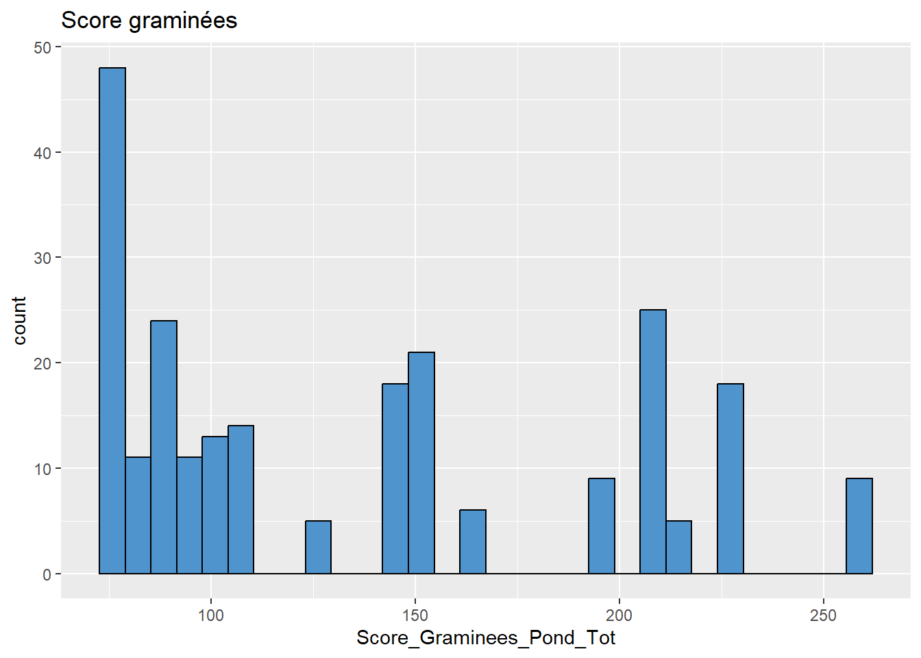
# Graminées
data %>%
ggplot(aes(x = Score_Graminees_Pond_Tot)) +
geom_histogram(colour="black", fill="steelblue3") +
labs(title = "Score graminées")
## `stat_bin()` using `bins = 30`. Pick better value with
## `binwidth`.
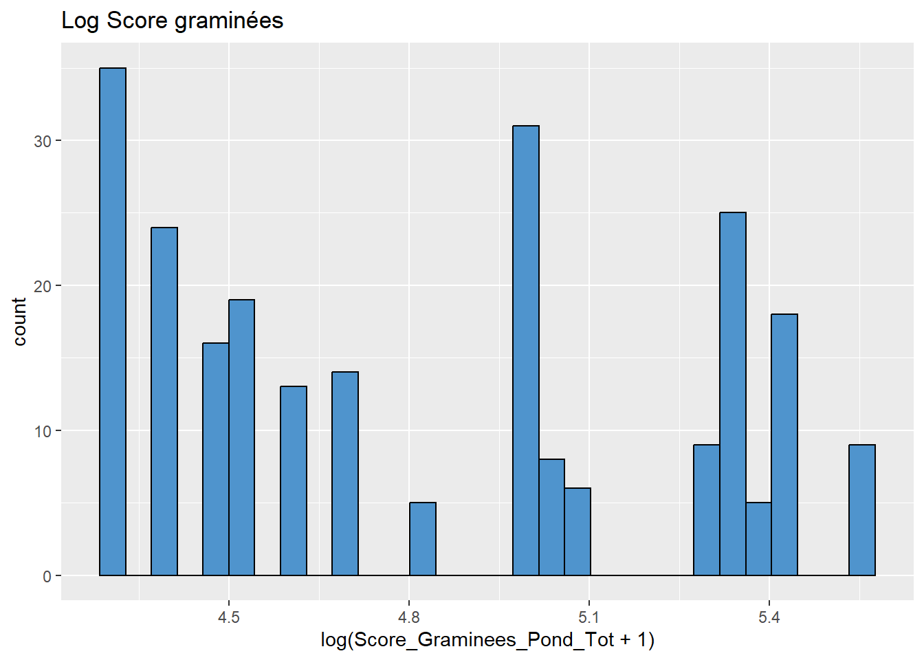
# Log Graminées
data %>%
  ggplot(aes(x = log(Score_Graminees_Pond_Tot+1))) +
  geom_histogram(colour="black", fill="steelblue3") +
  labs(title = "Log Score graminées")
## `stat_bin()` using `bins = 30`. Pick better value with
## `binwidth`.
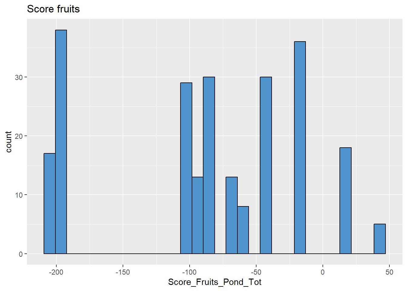
# Fruits
data %>%
  ggplot(aes(x = Score_Fruits_Pond_Tot)) +
  geom_histogram(colour="black", fill="steelblue3") +
  labs(title = "Score fruits")
## `stat_bin()` using `bins = 30`. Pick better value with
## `binwidth`.
# Fourmis
data %>%
  ggplot(aes(x = Score_Fourmis_Pond_Tot)) +
  geom_histogram(colour="black", fill="steelblue3") +
  labs(title = "Score fourmis")
## `stat_bin()` using `bins = 30`. Pick better value with
## `binwidth`.
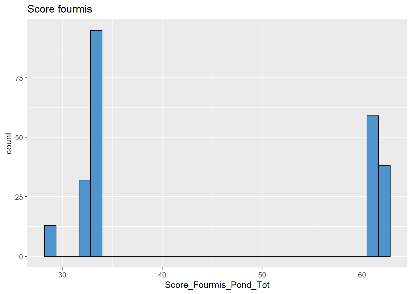
# pas bcp de données


# Noix
data %>%
  ggplot(aes(x = Score_Noix_Pond_Tot)) +
  geom_histogram(colour="black", fill="steelblue3") +
  labs(title = "Score noix")
## `stat_bin()` using `bins = 30`. Pick better value with
## `binwidth`.
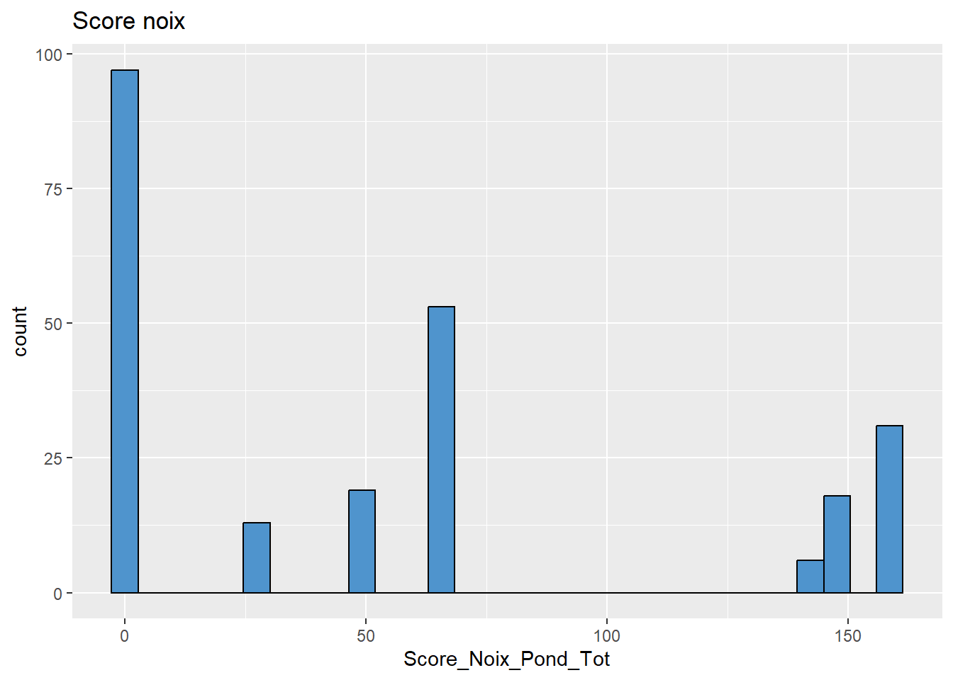
# pas bcp de données


### Les Y ###

# Pas de nouveau Y.

#### 6.2 - Homogénéité de la variance des Y####


# Masse moyenne des jeunes selon le secteur
data %>%
  ggplot(aes(Secteur, Weightx_Young_Corr_KG, col = Secteur)) +
  geom_boxplot(varwidth=T, alpha = 0.75) +
  labs(title="Masse moyenne des jeunes") +
  theme(legend.position="none")
## Warning: Removed 128 rows containing non-finite outside the
## scale range (`stat_boxplot()`).
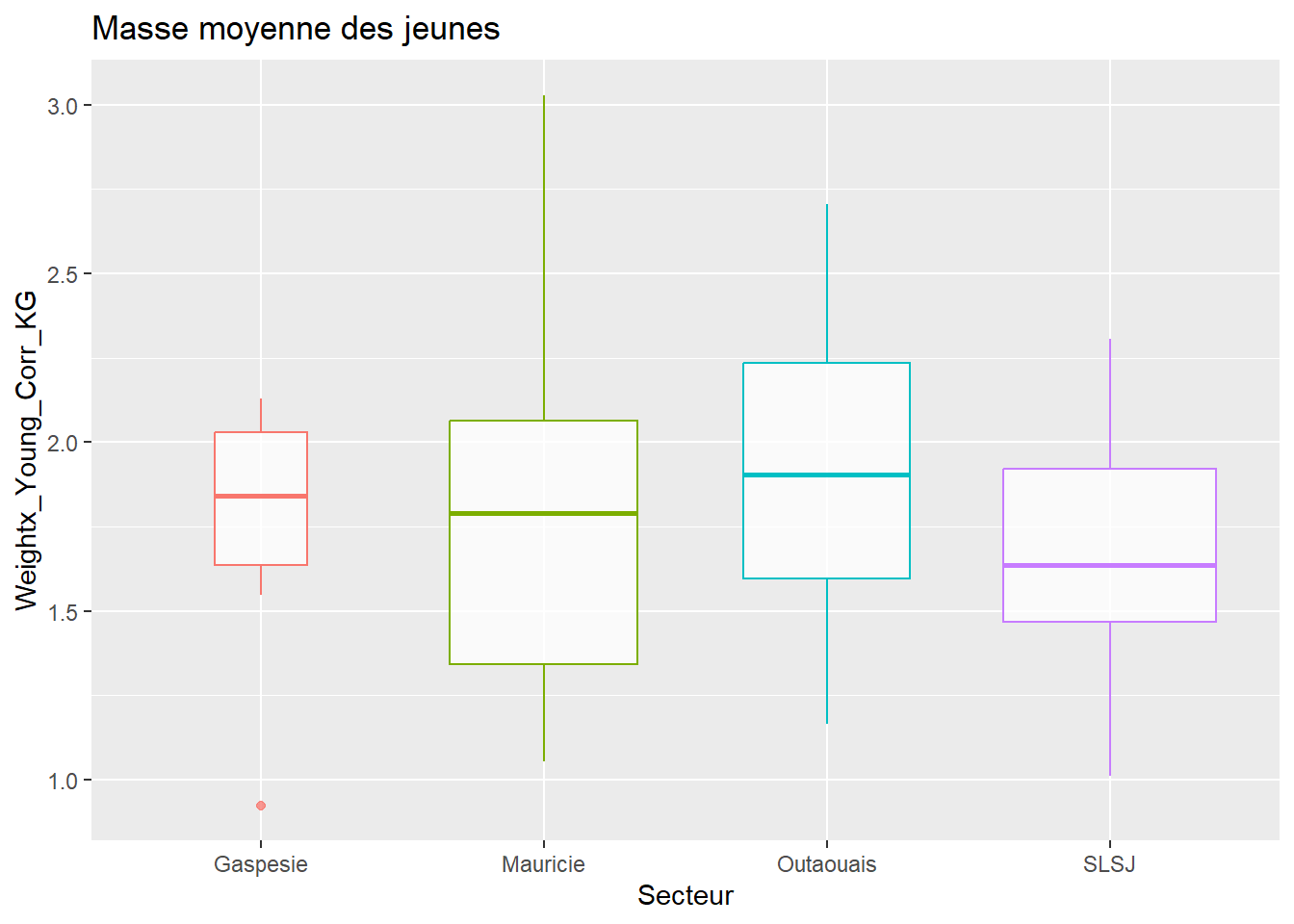
# Ok, un peu plus en Mauricie
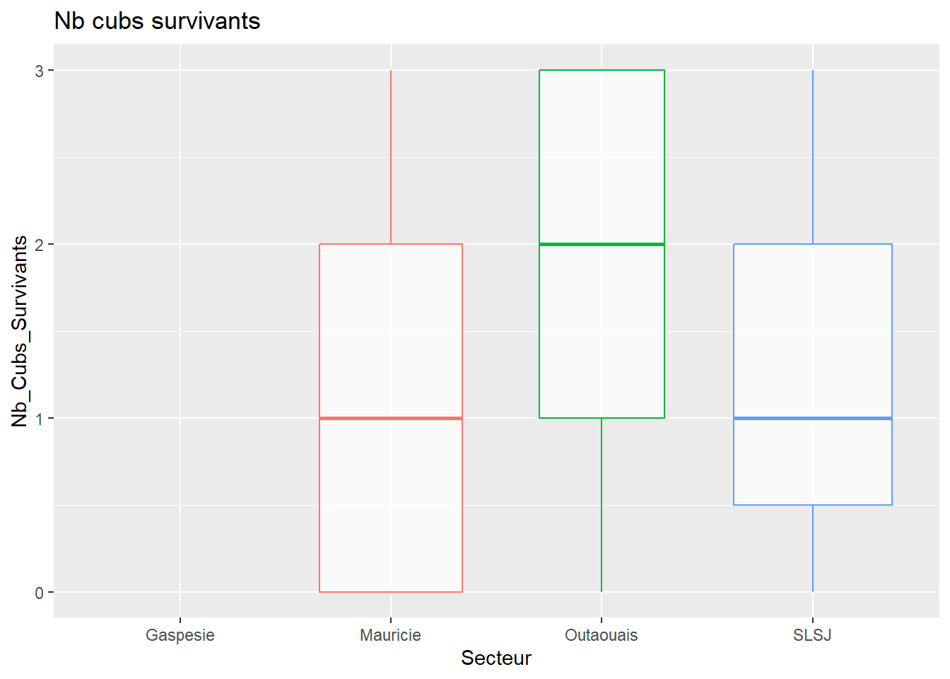
# Nombre de cubs qui survivent selon le secteur
data %>%
ggplot(aes(Secteur, Nb_Cubs_Survivants, col = Secteur)) +
geom_boxplot(varwidth=T, alpha = 0.75) +
labs(title="Nb cubs survivants") +
theme(legend.position="none")
## Warning: Removed 171 rows containing non-finite outside the
## scale range (`stat_boxplot()`).
#### 6.3 - Normalité des Y ####
# Pas de nouveau Y.
#### 6.4 - Problèmes de 0 dans les Y ####
# Pas de nouveau Y.
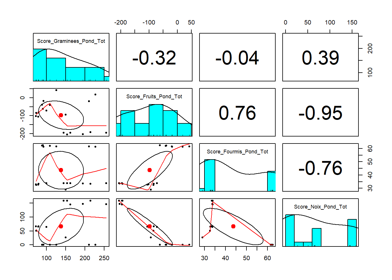
#### 6.5 - Colinéarité des X ####
as.data.frame(colnames(data))
##                  colnames(data)
## 1                     ID_Animal
## 2                       Secteur
## 3                   Year_Winter
## 4                    PCA1_Score
## 5                           Age
## 6                 Age_of_Youngs
## 7              Number_of_Youngs
## 8         Weightx_Young_Corr_KG
## 9  Den_Weight_an_1_KG_Corr_Cub1
## 10 Den_Weight_an_1_KG_Corr_Cub2
## 11 Den_Weight_an_1_KG_Corr_Cub3
## 12 Den_Weight_an_1_KG_Corr_Cub4
## 13           Nb_Cubs_Survivants
## 14                Nb_Cubs_Morts
## 15                 Ratio_Survie
## 16     Score_Graminees_Pond_Tot
## 17        Score_Fruits_Pond_Tot
## 18       Score_Fourmis_Pond_Tot
## 19          Score_Noix_Pond_Tot
etape6_5 = unique(data[,c(16:19)])

# Pearson
pairs.panels(etape6_5, method = "pearson")
# Spearman
pairs.panels(etape6_5, method = "spearman")

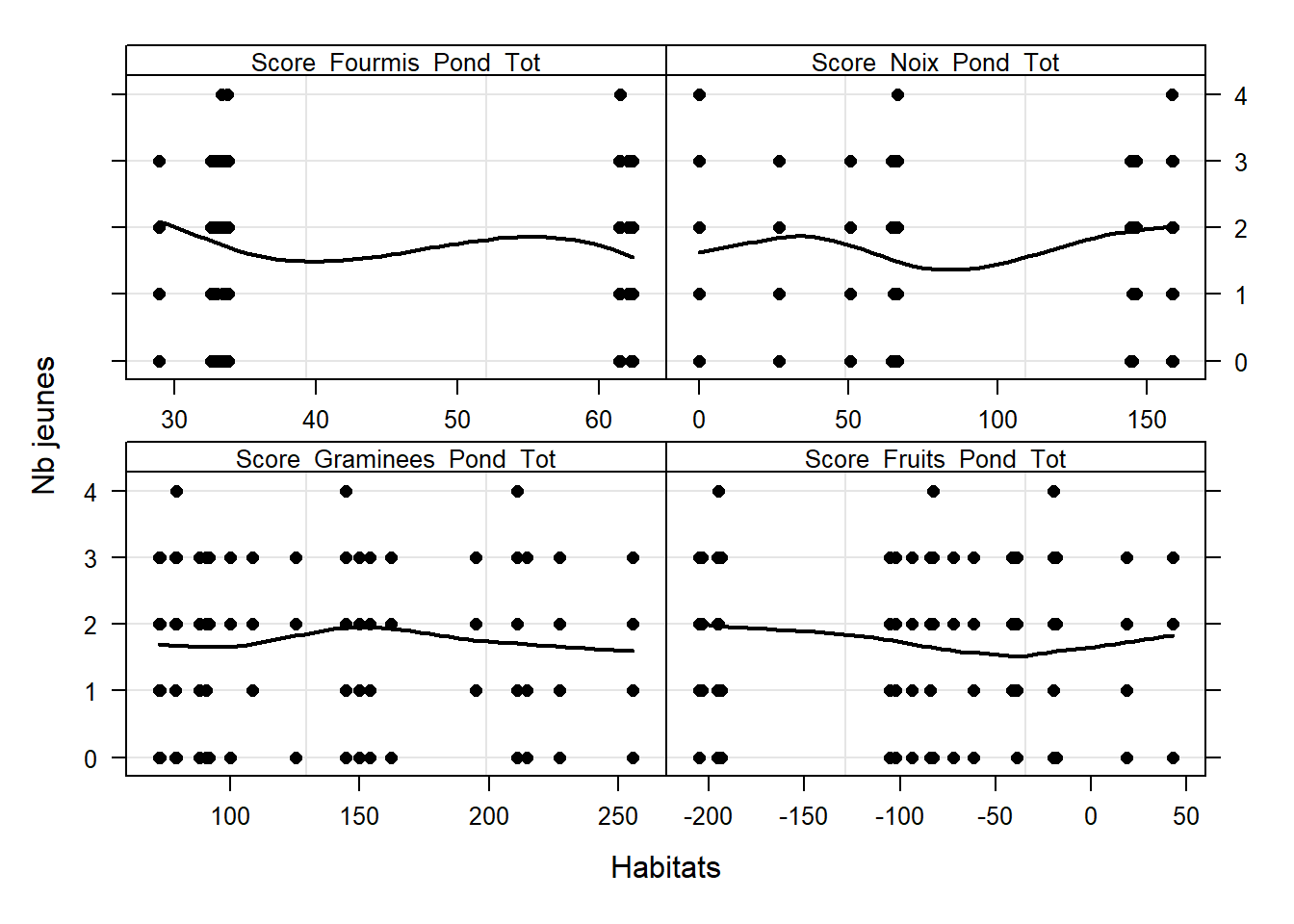
#### 6.6 - Relations entre les X et Y ####

# Nb jeunes

Z <- as.vector(as.matrix(data[, c(16:19)]))

Y10 <- rep(data$Number_of_Youngs, 4)

MyNames <- colnames(data)[16:19]

ID10 <- rep(MyNames, each = length(data$Number_of_Youngs))

ID11 <- factor(ID10, labels = MyNames,
               levels = MyNames)

xyplot(Y10 ~ Z | ID11, col = 1,
       strip = function(bg='white',...) strip.default(bg='white',...),
       scales = list(alternating = T,
                     x = list(relation = "free"),
                     y = list(relation = "same")),
       xlab = "Habitats",
       par.strip.text = list(cex = 0.8),
       ylab = "Nb jeunes",
       panel=function(x, y, subscripts,...){
         panel.grid(h =- 1, v = 2)
         panel.points(x, y, col = 1, pch = 16)
         panel.loess(x,y,col=1,lwd=2)
       })
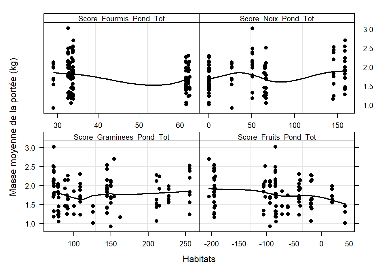
# Masse moyenne des jeunes

Z <- as.vector(as.matrix(data[, c(16:19)]))

Y10 <- rep(data$Weightx_Young_Corr_KG, 4)

MyNames <- colnames(data)[16:19]

ID10 <- rep(MyNames, each = length(data$Weightx_Young_Corr_KG))

ID11 <- factor(ID10, labels = MyNames,
               levels = MyNames)

xyplot(Y10 ~ Z | ID11, col = 1,
       strip = function(bg='white',...) strip.default(bg='white',...),
       scales = list(alternating = T,
                     x = list(relation = "free"),
                     y = list(relation = "same")),
       xlab = "Habitats",
       par.strip.text = list(cex = 0.8),
       ylab = "Masse moyenne de la portée (kg)",
       panel=function(x, y, subscripts,...){
         panel.grid(h =- 1, v = 2)
         panel.points(x, y, col = 1, pch = 16)
         panel.loess(x,y,col=1,lwd=2)
       })
# Nb survivants

Z <- as.vector(as.matrix(data[, c(16:19)]))

Y10 <- rep(data$Nb_Cubs_Survivants, 4)

MyNames <- colnames(data)[16:19]

ID10 <- rep(MyNames, each = length(data$Nb_Cubs_Survivants))

ID11 <- factor(ID10, labels = MyNames,
               levels = MyNames)

xyplot(Y10 ~ Z | ID11, col = 1,
       strip = function(bg='white',...) strip.default(bg='white',...),
       scales = list(alternating = T,
                     x = list(relation = "free"),
                     y = list(relation = "same")),
       xlab = "Habitats",
       par.strip.text = list(cex = 0.8),
       ylab = "Nb cubs survivants",
       panel=function(x, y, subscripts,...){
         panel.grid(h =- 1, v = 2)
         panel.points(x, y, col = 1, pch = 16)
         panel.loess(x,y,col=1,lwd=2)
       })

#### 6.7 - Interactions ####
# Pas d'interactions à regarder
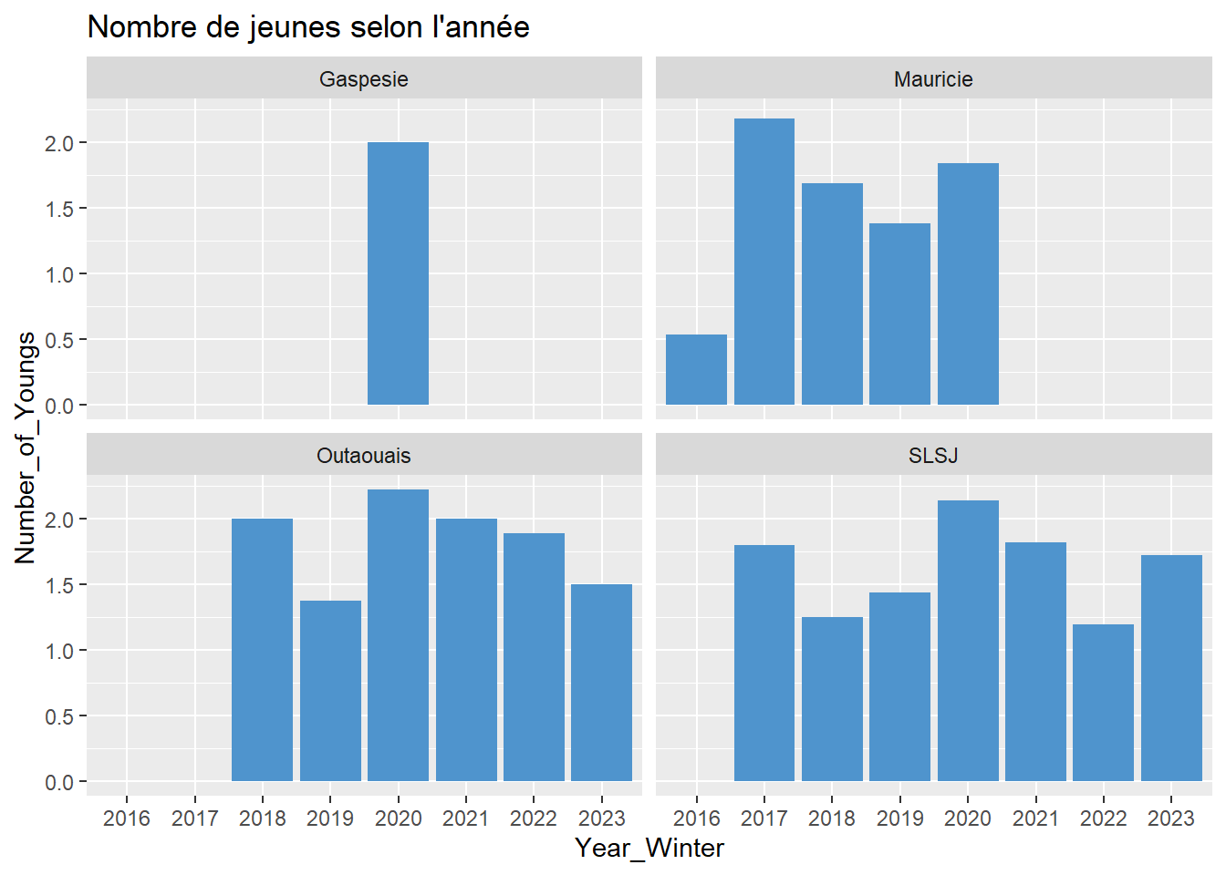
#### 6.8 - Indépendance des Y ####
# Les Y ne sont pas indépendants car il y a des répétitions au niveau des individus, du secteur et de l'année.
## Année/Secteur
# Nombre de jeunes selon l'année
data %>%
ggplot(aes(x = Year_Winter, y = Number_of_Youngs)) +
geom_bar(stat = "summary", position = "dodge", fun = "mean", fill = "steelblue3") +
labs(title = "Nombre de jeunes selon l'année") +
facet_wrap(~ Secteur)
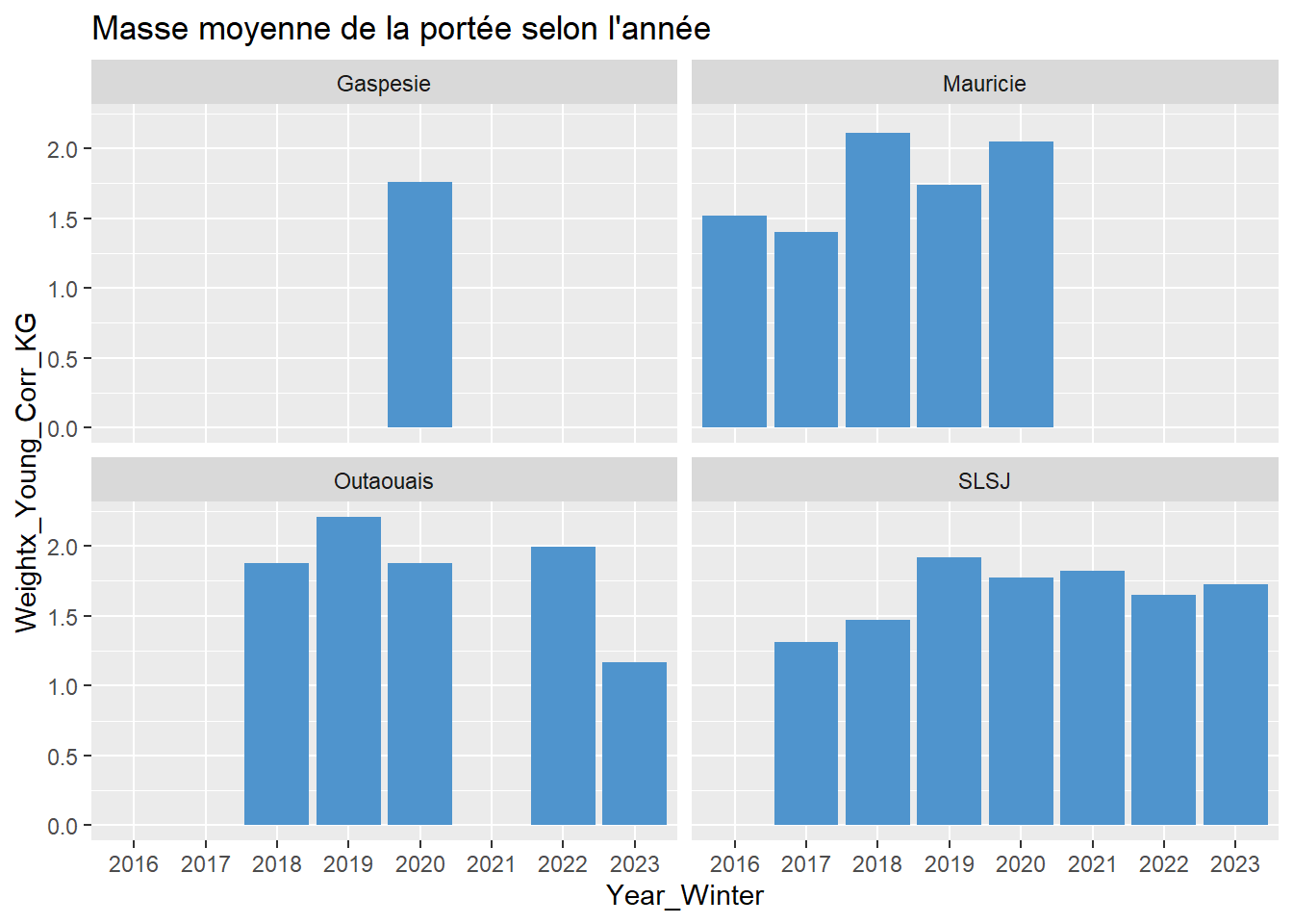
# Masse moyenne selon l'année
data %>%
  ggplot(aes(x = Year_Winter, y = Weightx_Young_Corr_KG)) +
  geom_bar(stat = "summary", position = "dodge", fun = "mean", fill = "steelblue3") +
  labs(title = "Masse moyenne de la portée selon l'année") +
  facet_wrap(~ Secteur)
## Warning: Removed 128 rows containing non-finite outside the
## scale range (`stat_summary()`).
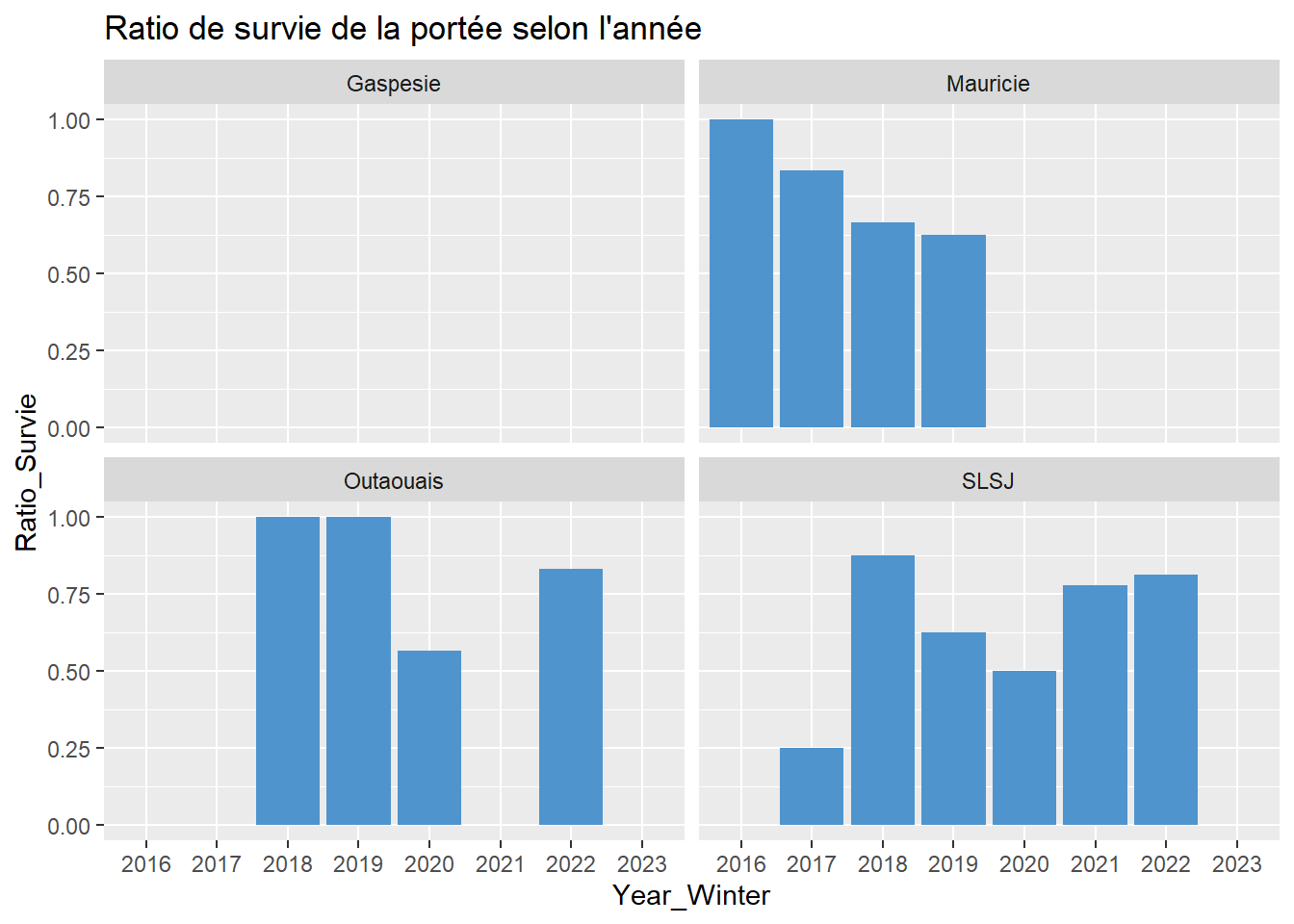
# Survie selon l'année
data %>%
  ggplot(aes(x = Year_Winter, y = Ratio_Survie)) +
  geom_bar(stat = "summary", position = "dodge", fun = "mean", fill = "steelblue3") +
  labs(title = "Ratio de survie de la portée selon l'année") +
  facet_wrap(~ Secteur)
## Warning: Removed 171 rows containing non-finite outside the
## scale range (`stat_summary()`).
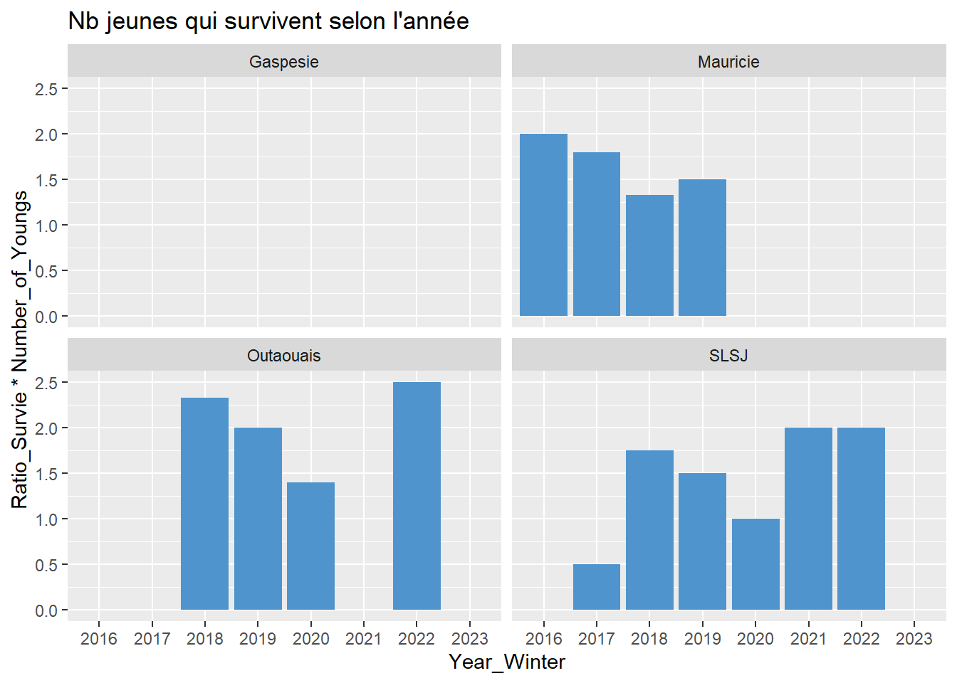
# Nb jeunes qui survivent selon l'année
data %>%
  ggplot(aes(x = Year_Winter, y = Ratio_Survie*Number_of_Youngs)) +
  geom_bar(stat = "summary", position = "dodge", fun = "mean", fill = "steelblue3") +
  labs(title = "Nb jeunes qui survivent selon l'année") +
  facet_wrap(~ Secteur)
## Warning: Removed 171 rows containing non-finite outside the
## scale range (`stat_summary()`).
#### 6.9 - Colinéarité des Y (si plusieurs Y) ####

# Pas de nouveau Y.