Chapter 9 Survival Analysis

These notes rely on the Survival Analysis in R DataCamp course, STHDA, BJC, Applied Survival Analysis Using R (Moore 2016), Emily Zabor, and Clark et al (1).

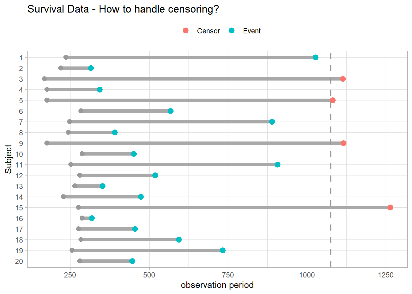
Survival analyses model time to event. They differ from linear regression in two respects. Event times are typically skewed right with many early events and few late ones, violating linear regression’s normality assumption. Survival analyses must also manage censoring, an unknown starting event (left censoring) and/or ending event (right censoring). Censuring occurs if the event does not take place by the end of the study window, or the subject is in some way lost to follow-up. In the figure below, subjects 3, 5, 9, and 15 either did not have the event or dropped out of the study. Censored observations do not reveal their total time to event, but they do reveal at least their minimum.

A typical survival analysis uses Kaplan-Meier (KM) plots to visualize survival curves, log-rank tests to compare survival curves among groups, and Cox proportional hazards regression to describe the effect of explanatory variables on survival. In R, use the survival package for modeling, survminer for visualization, and gtsummary for summarization.

library(scales)
library(survival)
library(survminer)
library(gtsummary)

9.1 Basics

Let \(T^*\) be a random variable representing the time until the event, and \(U\) be a random variable representing the time until (right) censoring. The observed value is whichever event comes first, \(T = \mathrm{min}(T^*, U)\). The lung data set is typical, with time representing \(T\) and status representing \(\delta = I[T^* < U]\) (1 = censored, 2 = event).

survival::lung %>% head()

##   inst time status age sex ph.ecog ph.karno pat.karno meal.cal wt.loss
## 1    3  306      2  74   1       1       90       100     1175      NA
## 2    3  455      2  68   1       0       90        90     1225      15
## 3    3 1010      1  56   1       0       90        90       NA      15
## 4    5  210      2  57   1       1       90        60     1150      11
## 5    1  883      2  60   1       0      100        90       NA       0
## 6   12 1022      1  74   1       1       50        80      513       0

Censoring sometimes occurs when subjects are monitored for a fixed period of time (Type I), the study is halted after a pre-specified level of events are reached (Type II), or the subject drops out for a reason other than the event of interest (random censoring).

You can specify the survival distribution function either as a survival function, \(S(t)\), or as a hazard function, \(h(t)\). Let \(F(t) = P(T \le t)\) be the cumulative risk function, the probability of the event occurring on or before time \(t\). \(S(t)\) is its complement, \(S(t) = 1 - F(t)\).

\[S(t) = P(T > t).\]

The hazard function is the instantaneous event rate at \(t\) given survival up to \(t\),

\[h(t) = \lim_{\delta \rightarrow 0}{\frac{P(t < T < t + \delta|T > t)}{\delta}}.\]

An instantaneous event rate has no intuitive appeal, but think of it in discrete time where \(\delta > 0\). \(h(t + \delta)\) is the conditional probability of an event at the discrete interval \(t + \delta\), conditioned on those at risk during that interval.

The survival and hazard functions are related by the multiplication rule, \(P(AB) = P(A|B)P(B)\). The event probability at \(t\), \(f(t) = F'(t)\), is the probability of the event at \(t\) given survival up to \(t\) multiplied by the probability of survival up to \(t\).

\[f(t) = h(t) S(t).\]

Again, in discrete terms, survival up to interval \(t\) is the sum product of the survival probabilities at each preceding period, \(S(t) = \Pi_{i = 1}^t [1 - h(t)]\). It is the complement of the cumulative risk.

Rearranging, \(h(t)dt = \frac{f(t)}{S(t)}dt\) describes the prognosis for a subject who has survived through time \(t\).

\(S(t)\) is also the negative exponent of the cumulative hazard function,

\[S(t) = e^{-H(t)}.\]

Use the survival function to estimate the mean survival time, \(E(T) = \int S(t)dt\), and median survival time, \(S(t) = 0.5\).

Take the exponential distribution as a quick example. It has a constant hazard, \(h(t) = \lambda\). The cumulative hazard is \(H(t) = \int_0^t \lambda du = \lambda t\). The survival function is \(S(t) = e^{-\lambda t}\). The probability of failure at time \(t\) is \(f(t) = \lambda e^{-\lambda t}\). The expected time to failure is \(E(t) = \int_0^\infty e^{-\lambda t} dt = 1 / \lambda\), and the median time to failure is \(S(t) = e^{-\lambda t} = .5\), or \(t_{med} = \log(2) / \lambda\).

There are parametric and non-parametric methods to estimate a survival curve. The usual non-parametric method is the Kaplan-Meier estimator. The usual parametric method is the Weibull distribution. In between is the most common way to estimate a survivor curve, the Cox proportional hazards model.

9.2 Kaplan-Meier

The Kaplan-Meier (KM) estimator for the survival function is the product over failure times of the conditional probabilities of surviving to the next failure time.

\[\hat{S}(t) = \prod_{i: t_i < t}{\frac{n_i - d_i}{n_i}}\]

where \(n_i\) is the number of subjects at risk at time \(i\) and \(d_i\) is the number incurring the event. I.e., \(\hat{S}(t)\) is the sum-product of the survival proportions at each time interval. The KM curve falls only when an event occurs, not when a subject is censored. Confidence limits are calculated using the “delta” method to obtain the variance of \(\log \hat{S}(t)\).

Calculate \(\hat{S}(t)\) with survival::survfit(). Data set lung records the status (1 = censored, 2 = dead) of 228 lung cancer patients. survfit() operates on a Surv object, created by Surv(). Explanatory variables can be defined as factors, but the event indicator must be numeric and coded as 0|1 or 1|2.¹¹

lung_1 <- survival::lung %>%
  mutate(sex = factor(sex, levels = c(1, 2), labels = c("Male", "Female")))

survfit() creates survival curves from a formula or from a previously fitted Cox model. If the confidence interval crosses zero, you can cap it, or specify the log-log transformation parameter conf.type = "log-log". This one doesn’t need it.

# km_fit <- survfit(Surv(time, status) ~ sex, data = lung, conf.type = "log-log")
km_fit <- survfit(Surv(time, status) ~ sex, data = lung_1)
km_fit

## Call: survfit(formula = Surv(time, status) ~ sex, data = lung_1)
## 
##              n events median 0.95LCL 0.95UCL
## sex=Male   138    112    270     212     310
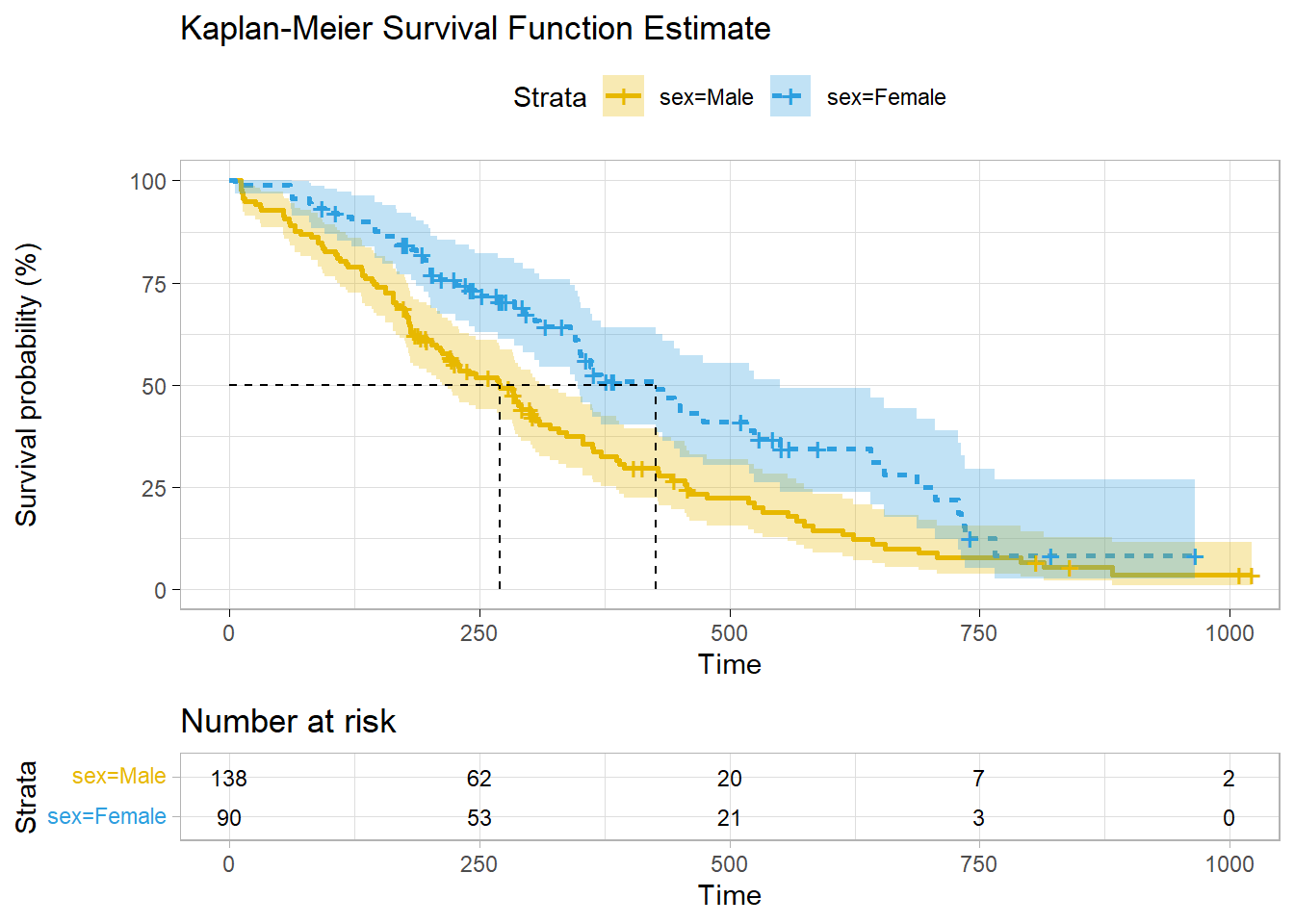
## sex=Female  90     53    426     348     550

112 of the 138 males and 53 of the 90 females died. The median survival times were 270 days for males and 426 days for females. The 95% CI is defined around the median time to event. Retrieve these values from the summary()$table object. E.g., summary(km_fit)$table[1, "0.95LCL"] = 212. You can also use summary() with the time parameter to estimate survival up until a point in time.

summary(km_fit, time = 300)

## Call: survfit(formula = Surv(time, status) ~ sex, data = lung_1)
## 
##                 sex=Male 
##         time       n.risk      n.event     survival      std.err lower 95% CI 
##     300.0000      49.0000      74.0000       0.4411       0.0439       0.3629 
## upper 95% CI 
##       0.5362 
## 
##                 sex=Female 
##         time       n.risk      n.event     survival      std.err lower 95% CI 
##     300.0000      43.0000      27.0000       0.6742       0.0523       0.5791 
## upper 95% CI 
##       0.7849

broom::tidy() summarizes the data by each event time in the data. At time t = 11, 3 of the 138 males at risk died, so \(S(11) = 1 - \frac{3}{138} = .978\). At t = 12, 1 of the 135 that remained died, so \(S(12) = S(11) \cdot \frac{1}{135} = .971\), and so on.

km_fit %>% broom::tidy()

## # A tibble: 206 × 9
##     time n.risk n.event n.censor estimate std.error conf.high conf.low strata  
##    <dbl>  <dbl>   <dbl>    <dbl>    <dbl>     <dbl>     <dbl>    <dbl> <chr>   
##  1    11    138       3        0    0.978    0.0127     1        0.954 sex=Male
##  2    12    135       1        0    0.971    0.0147     0.999    0.943 sex=Male
##  3    13    134       2        0    0.957    0.0181     0.991    0.923 sex=Male
##  4    15    132       1        0    0.949    0.0197     0.987    0.913 sex=Male
##  5    26    131       1        0    0.942    0.0211     0.982    0.904 sex=Male
##  6    30    130       1        0    0.935    0.0225     0.977    0.894 sex=Male
##  7    31    129       1        0    0.928    0.0238     0.972    0.885 sex=Male
##  8    53    128       2        0    0.913    0.0263     0.961    0.867 sex=Male
##  9    54    126       1        0    0.906    0.0275     0.956    0.858 sex=Male
## 10    59    125       1        0    0.899    0.0286     0.950    0.850 sex=Male
## # … with 196 more rows

Don’t construct your own ggplot - survminer does a good job plotting KM models. Vertical drops indicate events and vertical ticks indicate censoring.

ggsurvplot(
  km_fit,
  fun = "pct",
  linetype = "strata", # Change line type by groups
  pval = FALSE, 
  pval.method = TRUE,
  conf.int = TRUE,
  risk.table = TRUE,
  fontsize = 3, # used in risk table
  surv.median.line = "hv", # median horizontal and vertical ref lines
  ggtheme = theme_light(),
  palette = c("#E7B800", "#2E9FDF"),
  title = "Kaplan-Meier Survival Function Estimate"
)

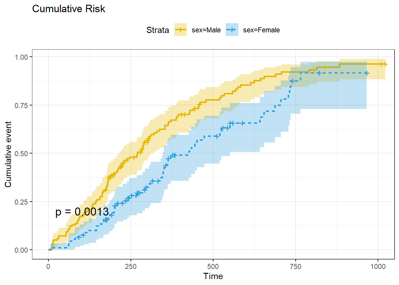
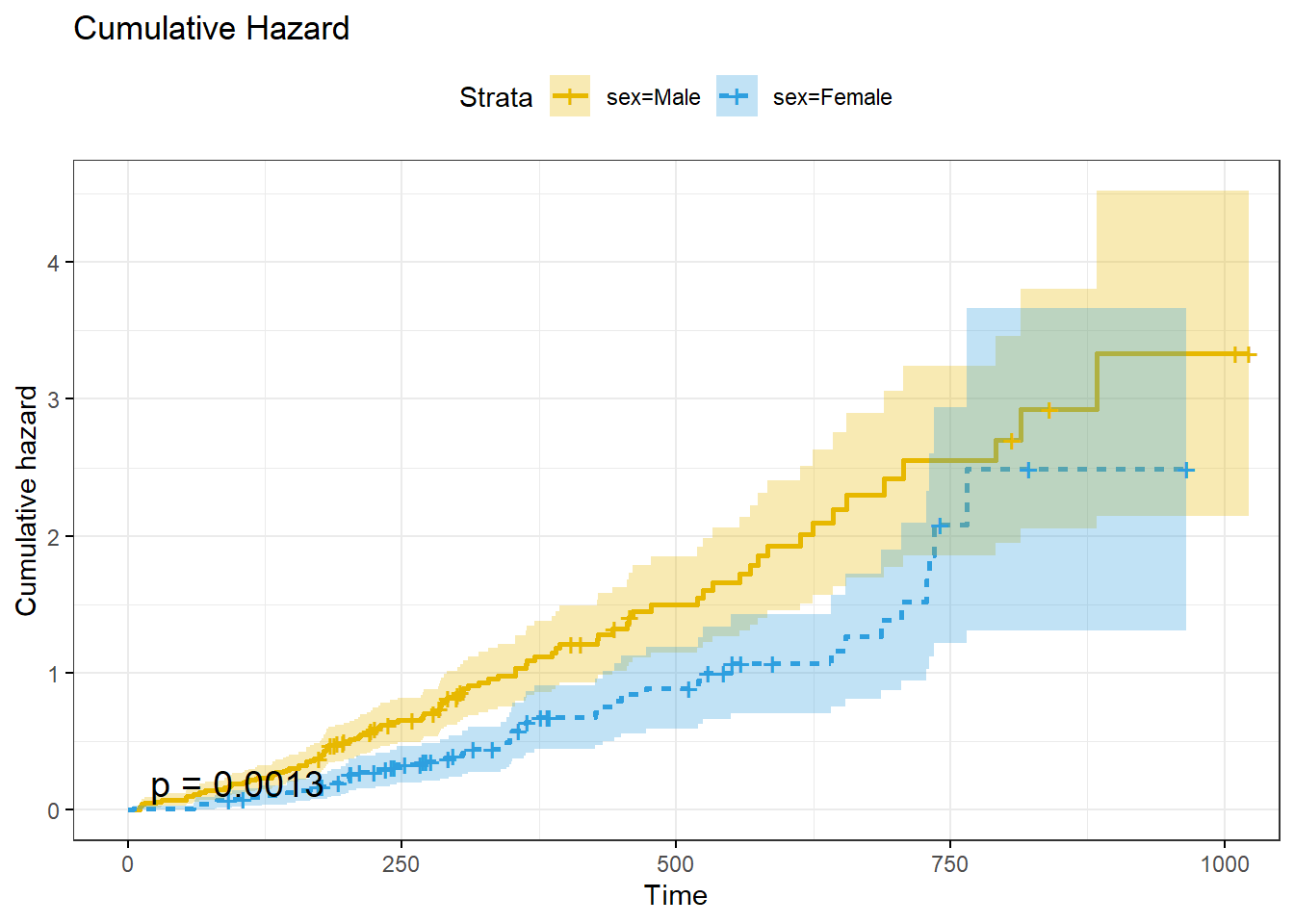
ggsurvplot() can also plot the cumulative risk function, \(F(t) = 1 - S(t)\), with parameter fun = "event", and the cumulative hazard function, \(H(t) = -\log S(t)\), with parameter fun = "cumhaz".

A KM analysis is valid under the following conditions:

• The event status consists of two states: event or censor,
• Left-censoring (unknown starting point) is minimal,
• Censoring causes are independent of the event,
• There are no secular trends (e.g., staggered starting times, or introduction of new therapies), and
• The amount and pattern of censorship is similar per group.

The first three assumptions relate to study design and cannot be tested, but secular trends can be tested by running KM tests for multiple time intervals, and censorship patterns can be tested by inspection.

9.3 Log-Rank Test

It is not obvious how to compare two survival distributions because they can cross, diverge, etc. When observations do not follow a parametric distribution function, compare them with the non-parametric log-rank test. The alternative hypothesis, termed the Lehmann alternative, is that one survival distribution is uniformly higher than the other, \(H_A : S_1(t) = [S_0(t)]^\psi\), or equivalently, the hazard functions are proportional, \(h_1(t) = \psi h_0(t)\), with \(H_A: \psi \ne 1\).

At each \(t\), you could construct a 2x2 contingency table between event/no-event and curves A and B.

	Curve A	Curve B	Total
Event	\(d_{Ai}\)	\(d_{Bi}\)	\(d_i\)
No Event	\(n_{Ai} - d_{0i}\)	\(n_{Bi} - d_{1i}\)	\(n_i - d_i\)
Total	\(n_{Ai}\)	\(n_{Bi}\)	\(n_i\)

Holding the margins as fixed, the probability of observing \(d_{Ai}\) events in curve A at time \(i\) follows a hypergeometric distribution.

\[f(d_{Ai} | n_{Ai}, n_{Bi}, d_i) = \frac{{{n_{Ai}}\choose{d_{Ai}}}{{n_{Bi}}\choose{d_{Bi}}}}{{n_i}\choose{d_i}}\]

The expected value is \(e_{Ai} = E(d_{Ai}) = \frac{d_i}{n_i} \cdot n_{0i}\) with variance \(v_{Ai} = Var(d_{Ai}) = d_{i} \cdot \frac{n_{Ai}}{n_i} \cdot \frac{n_{1i}}{n_i} \cdot \frac{n_i - d_i}{n_i - 1}\).

The log-rank test statistic is the sum of the differences between the observed and expected events, \(U_0 = \sum (d_{Ai} - e_{Ai})\), normalized by dividing by the square-root of its variance, \(V_0 = Var({U_0}) = \sum v_{Ai}\).

\[U = \frac{U_0}{\sqrt{V_0}} \sim N(0, 1)\]

\(U^2\) is a chi-square random variable with one degree of freedom.

\[U^2 = \frac{U_0^2}{V_0} \sim \chi_1^2\]

(km_diff <- survdiff(Surv(time, status) ~ sex, data = lung_1))

## Call:
## survdiff(formula = Surv(time, status) ~ sex, data = lung_1)
## 
##              N Observed Expected (O-E)^2/E (O-E)^2/V
## sex=Male   138      112     91.6      4.55      10.3
## sex=Female  90       53     73.4      5.68      10.3
## 
##  Chisq= 10.3  on 1 degrees of freedom, p= 0.001

The p-value for \(\chi_1^2\) = 10.3 is 1 - pchisq(km_diff$chisq, length(km_diff$n) - 1) = 0.001, so reject \(H_0\) that males and females have identical survival patterns.

9.4 Common Distributions

KM curves and logrank tests are univariate analyses. They describe survival as a function of a single categorical factor variable. Weibull and other parametric models describe the effect of multiple covariates. Fully-parametric models are less common than KM and the semi-parametric Cox model because they are less flexible, but if the process follows the parametric distribution these models are preferable because the estimated parameters provide clinically meaningful estimates of the effect¹².

9.4.1 Exponential

The exponential distribution (probability notes), \(T \sim \mathrm{Exp}(\lambda)\), is the easiest to use because its hazard function is time-independent.

\[\begin{eqnarray} \log h(t) &=& \alpha + \beta X \\ h(t) &=& e^{\left(\alpha + \beta X \right)} \\ &=& \lambda \end{eqnarray}\]

Interpret \(\alpha\) as the baseline log-hazard because when \(X\) is zero \(h(t) = e^\alpha\). The cumulative hazard is \(H(t) = \int_0^t \lambda dt = \lambda t\) and the corresponding survival function is

\[S(t) = e^{-H(t)} = e^{-\lambda t}.\]

The expected survival time is \(E(T) = \int_0^\infty S(t)dt = \int_0^\infty e^{-\lambda t} dt = 1 / \lambda.\) The median survival time is \(S(t) = e^{-\lambda t} = 0.5\), or \(t_{med} = \log(2) / \lambda\).

The survival curve is fit using maximimum likelihood estimation (MLE). My statistics notes explain MLE for the exponential distribution. Survival curve MLE is a little more complicated because of censoring. The likelihood \(L\) that \(\lambda\) produces the observed outcomes is the product of the probability densities for each observation because they are a sequence of independent variables. Let \(\delta_i = [1, 0]\) for unsensored and censored observations.

\[ L(\lambda; t_1, t_2, \dots, t_n) = \Pi_{i=1}^n f(t_i; \lambda)^{\delta_i} S(t_i; \lambda)^{1-\delta_i} \]

Substituting \(f(t) = h(t) S(t)\), and then substituting \(h(t) = \lambda\) and \(S(t) = e^{-\lambda t}\) and simplifying,

\[\begin{eqnarray} L(\lambda; t_1, t_2, \dots, t_n) &=& \Pi_{i=1}^n h(t_i; \lambda)^{\delta_i} S(t_i; \lambda) \\ &=& \Pi_{i=1}^n \lambda^{\delta_1} e^{-\lambda t_i} \\ &=& \lambda^{\sum \delta_i} \exp \left(-\lambda \sum_{i=1}^n t_i \right) \end{eqnarray}\]

Simplify the notation by letting \(d = \sum \delta_i\), the total number of events (or deaths or whatever), and \(V = \sum t_i\), the number of person-years (or days or whatever).

\[L(\lambda; t_1, t_2, \dots, t_n) = \lambda^d e^{-\lambda V}\]

This form is difficult to optimize, but the log of it is simple.

\[l(\lambda; t_1, t_2, \dots, t_n) = d \log(\lambda) - \lambda V\]

Maximize the log-likelihood equation by setting its derivative to zero and solving for \(\lambda\).

\[\begin{eqnarray} \frac{d}{d \lambda} l(\lambda; t_1, t_2, \dots, t_n) &=& \frac{d}{d \lambda} \left(d \log(\lambda) - \lambda V \right) \\ 0 &=& \frac{d}{\lambda} - V \\ \lambda &=& \frac{d}{V} \end{eqnarray}\]

\(\lambda\) is the reciprocal of the sample mean, person-years divided by failures.

The second derivative, \(-\frac{d}{\lambda^2}\), is approximately the negative of the variance of \(\lambda\).

\[V(\lambda) = d / V^2\]

9.4.2 Weibull

Although the exponential function is convenient, the Weibull distribution is more appropriate for modeling lifetimes.

Its hazard function is

\[\begin{eqnarray} h(t) &=& \alpha \lambda (\lambda t)^{\alpha - 1} \\ &=& \alpha \lambda^\alpha t^{\alpha-1} \end{eqnarray}\]

The cumulative hazard function is \(H(t) = (\lambda t)^\alpha\) and the corresponding survival function is

\[S(t) = e^{-(\lambda t)^\alpha}.\]

The exponential distribution is a special case of the Weibull where \(\alpha = 1\). The expected survival time is \(E(t) = \frac{\Gamma (1 + 1 / \alpha)}{\lambda}\). The median survival time is \(t_{med} = \frac{[\log(2)]^{1 / \alpha}}{\lambda}\).

To measure the effects of covariates, it is preferable to substitute \(\sigma = 1 / \alpha\) and \(\mu = -\log \lambda\) so

\[ h(t) = \frac{1}{\sigma} e^{-\frac{\mu}{\sigma}} t^{\frac{1}{\sigma} - 1} \]

and

\[ S(t) = e^{-e^{-\mu/\sigma}t^{1/\sigma}} \]

The log of the negative log of \(S\), \(\log[-\log(S_i)] = \alpha \log(\lambda) + \alpha \log(t_i) = \frac{\mu}{\sigma} + \frac{1}{\sigma} \log(t_i)\) is a linear function, so you can use it to determine whether the Weibull function is appropriate for your analysis. Return to the lung data set introduced in Kaplan-Meier section. Use the Kaplan-Meier estimate of the survival distribution to extract the survival estimates and each time, transform them to conform to the above equation, and fit a linear model.

km_fit_1 <- survfit(Surv(time, status) ~ 1, data = lung)
log_log_s <- log(-log(km_fit_1$surv))
log_t <- log(km_fit_1$time)

km_fit_1_lm <- lm(log_log_s ~ log_t)
km_fit_1_lm %>%
  broom::augment() %>%
  ggplot(aes(x = log_t)) +
  geom_point(aes(y = log_log_s)) +
  geom_line(aes(y = .fitted), linetype = 2, color = "goldenrod") +
  theme_light()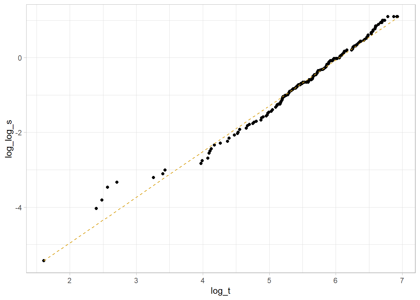

This is a decent fit. The coefficient estimates are

coef(km_fit_1_lm)

## (Intercept)       log_t 
##   -7.402713    1.223005

so \(\mu = -\frac{-7.403}{1.223} = -6.053\) and \(\sigma = \frac{1}{1.223} = {0.818}\).

Compare two Weibull distributions using the accelerated failure time (AFT) model. This model assumes the survival time for the treatment group is a multiple, \(e^\gamma\), of the control group survival time. The survival distributions in the AFT model are related as \(S_1(t) = S_0(e^{-\gamma}t)\) and the hazards are related by \(h_1(t) = e^{-\gamma}h_0(e^{-\gamma}t)\). In the case of the Weibull distribution, the relationship is \(h_1(t) = e^{-\frac{\gamma}{\sigma}}h_0(t)\). Fit a Weibull model with survreg() (recall KM is fit with survfit()). Return to the original model using the lung data set to compare survival between males and females.

dat <- lung %>% mutate(sex = factor(sex, levels = c(1, 2), labels = c("Male", "Female")))
wb_fit <- survreg(Surv(time, status) ~ sex, data = dat, dist = "weibull")
summary(wb_fit) 

## 
## Call:
## survreg(formula = Surv(time, status) ~ sex, data = dat, dist = "weibull")
##               Value Std. Error     z       p
## (Intercept)  5.8842     0.0720 81.76 < 2e-16
## sexFemale    0.3956     0.1276  3.10  0.0019
## Log(scale)  -0.2809     0.0619 -4.54 5.7e-06
## 
## Scale= 0.755 
## 
## Weibull distribution
## Loglik(model)= -1148.7   Loglik(intercept only)= -1153.9
##  Chisq= 10.4 on 1 degrees of freedom, p= 0.0013 
## Number of Newton-Raphson Iterations: 5 
## n= 228

\(\hat{\gamma} = 0.3956\), meaning females have longer times until death by a factor of \(e^{\hat{\gamma}} = e^{0.3956} = 1.49\). The scale parameter estimate is \(\hat\sigma = 0.755\), so the log proportional hazards is \(\hat\beta = -\frac{\hat\gamma}{\hat\sigma} = \frac{0.3956}{0.755} = 0.524\).

The survival curve estimate is \(\hat{S}(t) = e^{-e^{-\hat\mu/\hat\sigma}t^{1/\hat\sigma}}\), but \(\hat\alpha = 1 / \hat\sigma\).

new_dat <- expand.grid(
  sex = levels(dat$sex), 
  survival = seq(.01, .99, by = .01)
  ) %>%
  mutate(
    pred = map2(sex, survival, 
                ~predict(wb_fit, type = "quantile", p = 1 - .y, se = TRUE, 
                         newdata = data.frame(sex = .x))),
    t = map_dbl(pred, ~pluck(.x, "fit")),
    se = map_dbl(pred, ~pluck(.x, "se.fit")),
    ucl = t + 1.96 * se,
    lcl = t - 1.96 * se
  )

palette_sex <- c("#E7B800", "#2E9FDF")
names(palette_sex) <- c("Male", "Female")

new_dat %>%
  ggplot(aes(y = survival)) +
  geom_line(aes(x = t, color = sex)) +
  geom_ribbon(aes(xmin = lcl, xmax = ucl, fill = sex), alpha = 0.2) +
  scale_color_manual(values = palette_sex) +
  scale_fill_manual(values = palette_sex) +
  theme_light()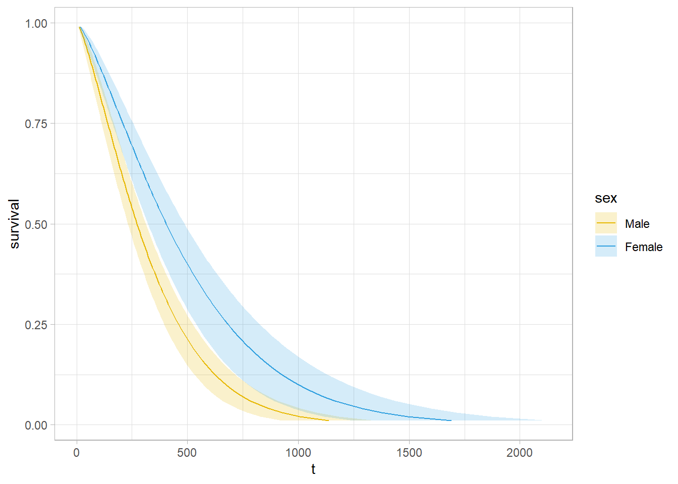

Use predict() to get survival expectations.

# 90% of subjects fail by time 
wb_fit %>% predict(type = "quantile", p = .9, newdata = data.frame(sex = levels(dat$sex)))
##         1         2 
##  674.4717 1001.7539

# Median survival times
predict(wb_fit, type = "quantile", p = 1 - 0.5, newdata = data.frame(sex = levels(dat$sex)))

##        1        2 
## 272.4383 404.6370

You can fit other models with the dist = c("lognormal", "exponential") parameter.

9.5 Cox

The Cox proportional hazards model expresses the expected hazard, \(h(t)\), as an unspecified baseline hazard, \(h_0(t)\), multiplied by the exponential of a linear combination of parameters, \(\psi = e^{X\beta}\).

\[h(t) = h_0(t) \cdot e^{X \beta} = \psi h_0(t).\]

\(h(t)\) is unspecified because it cancels out of the model. To see this, consider a hypothetical data set where 6 participants are assumed to fall into one of two hazards: participants 1, 2, and 3 have \(h_0\) and 4, 5, and 6 have \(\psi h_0\). Working through the event occurrences, the survival function is the product of each of the failure probabilities. Suppose participant 1 fails first. \(p_1 = \frac{h_0(t_1)}{3 \cdot h_0(t_1) + 3 \psi \cdot h_0(t_1)}\). Suppose participant 2 censors, then participant 4 fails. \(p_2 = \frac{\psi h_0(t_2)}{1 \cdot h_0(t_2) + 3 \psi \cdot h_0(t_2)}\). Now participant 3 fails. \(p_3 = \frac{h_0(t_3)}{1 \cdot h_0(t_3) + 2 \psi \cdot h_0(t_3)}\). Notice how \(h_0(t)\) cancels in each ratio. The partial likelihood is the product of the failure probabilities, \(L(\psi) = \frac{\psi}{(3 + 3 \psi)(1 + 3 \psi)(1 + 2 \psi)}\).

Find the value of \(\psi\) that maximizes \(L(\psi)\). \(L(\psi)\) is difficult to optimize, but its log is easier. \(l(\beta) = X \beta - \log (3 + 3 e^{X\beta}) - \log (1 + 3 e^{X\beta}) - \log (1 + 2 e^{X\beta})\). A function searches for the \(\beta\) producing the global max.

The proportionality of the model comes from the lack of time dependence in the \(X\) variables. The ratio of the hazard functions of two individuals is

\[\frac{h_i(t)}{h_{i'}(t)} = \frac{h_0(t) \cdot e^{X_i \beta}}{h_0(t) \cdot e^{X_{i'} \beta}}\]

There are three ways to test \(H_0 : \beta = 0\): the Wald test, the score test, and the likelihood ratio test.

• The Wald test statistic is \(Z = \hat{\beta} / se({\hat{\beta}})\). Calculate \(se({\hat{\beta}})\) from the second derivative of \(l(\beta)\). As with other Wald tests, the square of this standard normal random variable is distributed chi-square, so you can equivalently test whether \(Z^2 > \chi_{\alpha, 1}^2\).

• The score test compares the slope of \(l(\beta)\) at \(\beta = 0\) to 0. The test statistic is normally distributed, and again, its square is distributed chi-square.

• The likelihood ratio test statistic equals \(2 [l(\beta = \hat{\beta}) - l(\beta = 0)]\). It has a chi-square distribution with one degree of freedom.

The Cox proportional hazards model is analogous to the logistic regression model. Rearranging \(h(t) = h_0(t) \cdot e^{X \beta}\),

\[\ln \left[ \frac{h(t)}{h_0(t)} \right] = X \beta.\]

Whereas logistic regression predicts the log odds of the response, Cox regression predicts the log relative hazard (relative to the unspecified baseline) of the response. \(\beta\) is the change in the log of the relative hazard associated with a one unit change in \(X\). Its antilog is the hazard ratio (HR). A positive \(e^{\beta_j}\) means the hazard increases with the covariate.

\[ \begin{eqnarray} (x_b - x_a) \beta &=& \ln \left[ \frac{h_b(t)}{h_0(t)} \right] - \ln \left[ \frac{h_a(t)}{h_0(t)} \right] \\ \beta &=& \ln \left[ \frac{h_b(t)}{h_a(t)} \right] \\ e^\beta &=& \frac{h_b(t)}{h_a(t)} \\ &=& \mathrm{HR} \end{eqnarray} \]

Fit a Cox proportional hazards model with coxph().

dat <- lung %>% 
  mutate(
    sex = factor(sex, levels = c(1, 2), labels = c("Male", "Female")),
    ph.ecog = factor(ph.ecog, levels = c(0, 1, 2, 3), 
                     labels = c("asymptomatic", "ambulatory", "bedlow", "bedhigh"))
  )

cox_fit <- coxph(Surv(time, status) ~ sex, data = dat)
summary(cox_fit)

## Call:
## coxph(formula = Surv(time, status) ~ sex, data = dat)
## 
##   n= 228, number of events= 165 
## 
##              coef exp(coef) se(coef)      z Pr(>|z|)   
## sexFemale -0.5310    0.5880   0.1672 -3.176  0.00149 **
## ---
## Signif. codes:  0 '***' 0.001 '**' 0.01 '*' 0.05 '.' 0.1 ' ' 1
## 
##           exp(coef) exp(-coef) lower .95 upper .95
## sexFemale     0.588      1.701    0.4237     0.816
## 
## Concordance= 0.579  (se = 0.021 )
## Likelihood ratio test= 10.63  on 1 df,   p=0.001
## Wald test            = 10.09  on 1 df,   p=0.001
## Score (logrank) test = 10.33  on 1 df,   p=0.001

A negative coefficient estimator means the hazard decreases with increasing values of the variable. Females have a log hazard of death equal to coef(cox_fit)[1] = -0.5310 of that of males. The exponential is the hazard ratio, the effect-size of the covariate. Being female reduces the hazard by a factor of exp(coef(cox_fit)[1]) = 0.588 (41.2%). I.e., at any given time, 0.588 times as many females die as males.

The last section of the summary object is the three tests for the overall significance of the model. These three methods are asymptotically equivalent. The Likelihood ratio test has better behavior for small sample sizes, so it is generally preferred.

Use gtsummary to present the results.

cox_fit %>%
  tbl_regression(exponentiate = TRUE)

Characteristic	HR1	95% CI1	p-value
sex
Male	—	—
Female	0.59	0.42, 0.82	0.001
1 HR = Hazard Ratio, CI = Confidence Interval

A multivariate analysis works the same way. Here is the Cox model with two additional covariates: age and ph.ecog.

cox_fit_2 <- coxph(Surv(time, status) ~ age + sex + ph.ecog, data = dat)
summary(cox_fit_2)

## Call:
## coxph(formula = Surv(time, status) ~ age + sex + ph.ecog, data = dat)
## 
##   n= 227, number of events= 164 
##    (1 observation deleted due to missingness)
## 
##                        coef exp(coef)  se(coef)      z Pr(>|z|)    
## age                0.010795  1.010853  0.009312  1.159  0.24637    
## sexFemale         -0.545831  0.579360  0.168228 -3.245  0.00118 ** 
## ph.ecogambulatory  0.410048  1.506890  0.199604  2.054  0.03995 *  
## ph.ecogbedlow      0.903303  2.467741  0.228078  3.960 7.48e-05 ***
## ph.ecogbedhigh     1.954543  7.060694  1.029701  1.898  0.05767 .  
## ---
## Signif. codes:  0 '***' 0.001 '**' 0.01 '*' 0.05 '.' 0.1 ' ' 1
## 
##                   exp(coef) exp(-coef) lower .95 upper .95
## age                  1.0109     0.9893    0.9926    1.0295
## sexFemale            0.5794     1.7260    0.4166    0.8056
## ph.ecogambulatory    1.5069     0.6636    1.0190    2.2284
## ph.ecogbedlow        2.4677     0.4052    1.5782    3.8587
## ph.ecogbedhigh       7.0607     0.1416    0.9383   53.1289
## 
## Concordance= 0.637  (se = 0.025 )
## Likelihood ratio test= 30.87  on 5 df,   p=1e-05
## Wald test            = 31.43  on 5 df,   p=8e-06
## Score (logrank) test = 33.56  on 5 df,   p=3e-06

The p-values for all three overall tests (likelihood, Wald, and score) are significant, indicating that the model is significant (not all \(\beta\) values are 0).

A landmark analysis measures survival after a milestone period. E.g., I data set may have survival times after a disease onset, but a treatment typically starts after 90 days. In that case, you want to subset the persons surving at least 90 days and then subtract 90 from all the times. In a KM analysis manually adjust the data. In coxph() use the subset argument.

coxph(
  Surv(time, status) ~ age + sex + ph.ecog, 
  subset = time > 90, 
  data = dat
)

Visualize the fitted Cox model for each risk group. Function survfit() estimates survival at the mean values of covariates by default. That’s usually not useful, so instead pass a dataframe with test cases into the newdata argument.

# Predictions will be for all levels of sex and ph.ecog, but only at the median
# age.
new_data <- expand.grid(
    sex = unique(dat$sex),
    age = median(dat$age),
    ph.ecog = levels(dat$ph.ecog)
) %>% mutate(
  # strata is our key to join back to the fitted values.
  strata = as.factor(row_number())
)

# Create fitted survival curves at the covariate presets.
lung_pred_0 <- survfit(cox_fit_2, newdata = new_data, data = dat)

# `surv_summary()` is like `summary()` except that it includes risk table info,
# confidence interval attributes, and pivots the strata longer.
lung_pred_1 <- surv_summary(lung_pred_0)

# The cases are labeled "strata", but `survsummary()` doesn't label what the 
# strata are! Get it from new_data.
lung_pred_2 <- lung_pred_1 %>% inner_join(new_data, by = "strata")

# Now use ggplot() just like normal.
lung_pred_2 %>%
  ggplot(aes(x = time, y = surv, color = sex, fill = sex)) +
  geom_line() +
  geom_ribbon(aes(ymin = lower, ymax = upper), alpha = 0.4) +
  facet_wrap(facets = vars(ph.ecog)) +
  theme_light() +
  labs(title = "Cox fitted model",
       subtitle = "Age held at median.")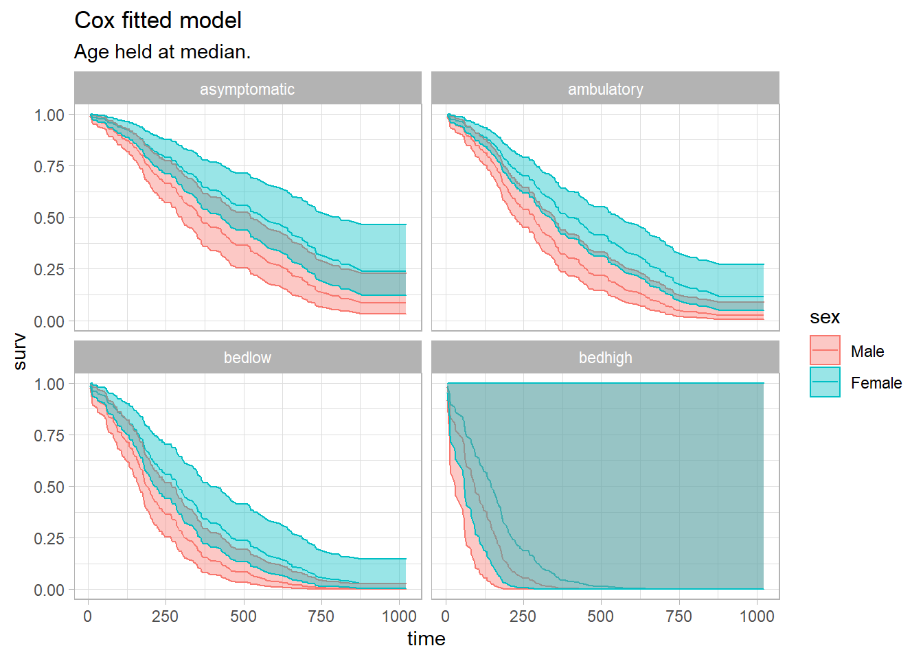

If a covariate changes over time, you need to modify the underlying data set. tmerge() lengthens the data set for the relevant time spans for the time-dependent covariate. Helper functions event() and tdc() modify the outcome and time-dependent covariates.

The BMT data set from the SemiCompRisks package is a good example. T1 and delta1 are the time and event indicator variables. TA and deltaA are time and event indicators for a secondary disease.

data(BMT, package = "SemiCompRisks")

dat <- BMT %>%
  rowid_to_column("subject_id") %>%
  select(subject_id, T1, delta1, TA, deltaA)

dat %>% filter(subject_id %in% c(1, 2, 15, 18))

##   subject_id   T1 delta1   TA deltaA
## 1          1 2081      0   67      1
## 2          2 1602      0 1602      0
## 3         15  418      1  418      0
## 4         18  156      1   28      1

tmerge() merges two data sets, usually the same ones, and expands the time/event vars.

dat_2 <- tmerge(
  data1 = dat,
  data2 = dat,
  id = subject_id,
  death = event(T1, delta1),
  agvhd = tdc(TA)
)

dat_2 %>% filter(subject_id %in% c(1, 2, 15, 18))

##   subject_id   T1 delta1   TA deltaA tstart tstop death agvhd
## 1          1 2081      0   67      1      0    67     0     0
## 2          1 2081      0   67      1     67  2081     0     1
## 3          2 1602      0 1602      0      0  1602     0     0
## 4         15  418      1  418      0      0   418     1     0
## 5         18  156      1   28      1      0    28     0     0
## 6         18  156      1   28      1     28   156     1     1

Define the Cox model Surv object with the start and end times.

dat_2 %>% 
  coxph(Surv(time = tstart, time2 = tstop, event = death) ~ agvhd, data = .) %>% 
  gtsummary::tbl_regression(exp = TRUE)

Characteristic	HR1	95% CI1	p-value
agvhd	1.40	0.81, 2.43	0.2
1 HR = Hazard Ratio, CI = Confidence Interval

From Emily Zabor’s tutorial, use a landmark analysis to visualize a covariate and Cox for modeling.

The Cox model is valid under certain conditions.

• Censoring event causes should be independent of the event.
• There is a multiplicative relationship between the predictors and the hazard.
• The hazard ratio is constant over time.

9.6 Discrete Time

Cox extended the proportional hazards model to discrete times using logistic regression. Times are discrete when the events they mark refer to an interval rather than an instant (e.g., grade when dropped out of school).

Recall that for continuous times the Cox proportional hazards model fits \(h(t) = h_0(t) \cdot e^{X\beta}\), and taking the log and rearranging describes a linear relationship between the log relative hazard and the predictor variables, \(\ln \left[ \frac{h(t)}{h_0(t)} \right] = X\beta\). The antilog of \(\beta\) is a hazard ratio (relative risk).

Fit a discrete-time model to an expanded data set that has one record for each subject and relevant time interval, and a binary variable representing the status. E.g., if event times in the data set occur in the range [16, 24] and individual i has the event at t = 20, then i’s record would expand to five rows with t = [16, 20] and status = [0, 0, 0, 0, 1].

The discrete-time model fits either a) the logit of the hazard at period t, \(\ln \left[ \frac{h(t)}{1 - h(t)} \right] = \alpha + X \beta\), or the complementary log-log, \(\ln (- \ln (1 - h(t))) = \alpha + X \beta\).¹³ \(\alpha = \mathrm{logit}\hspace{1mm}h_0(t)\) is the logit of the baseline hazard. The model treats time as discrete by introducing one parameter \(\alpha_j\) for the \(j\) possible event times in the data set (that’s why you expand the data set). The model fit is regular logistic regression.

Whereas the antilog of \(\beta\) in the continuous model is the hazard ratio, in the logit model it is the hazard odds ratio. The Cox and logit models converge as \(t \rightarrow 0\) because \(\log(h(t) \sim \log \frac{h(t)}{1 - h(t)}\) as \(t \rightarrow 0\). In the the complementary log-log model, the antilog of \(\beta\) is the hazard ratio, just as in Cox. Specify the link function in glm with family = binomial(link = "cloglog").

9.7 Case Study: KM + Cox

The guidelines for reporting the Kaplan-Meier test are from Laerd’s Kaplan-Meier using SPSS Statistics (Laerd 2015). The data is from survival::cancer. A researcher investigates differences in all-cause mortality between men and women diagnosed with advanced lung cancer. 227 participants aged 39 to 82 are monitored up to three years until time of death. The participants are segmented into three groups according to their ECOG performance score: asymptomatic, symptomatic but completely ambulatory, and bedridden at least part of the day. The study results are controlled for participant age.

(t1 <- cs_dat %>%
  mutate(status = factor(status, levels = c(1, 2), labels = c("censored", "died"))) %>%
  tbl_summary(by = "ph.ecog", include = vars(time, status, ph.ecog, age)) %>%
  add_overall())

## ! Use of `vars()` is now deprecated and support will soon be removed. Please replace calls to `vars()` with `c()`.

Characteristic	Overall, N = 2271	Asymptomatic, N = 631	Ambulatory, N = 1131	Bedridden, N = 511
time	259 (168, 399)	303 (224, 438)	243 (177, 426)	180 (100, 301)
status
censored	63 (28%)	26 (41%)	31 (27%)	6 (12%)
died	164 (72%)	37 (59%)	82 (73%)	45 (88%)
age	63 (56, 69)	61 (56, 68)	63 (55, 68)	68 (60, 73)
1 Median (IQR); n (%)

9.7.1 KM

KM survival analyses require 1) binary outcomes (event or censoring), 2) defined times to events, 3) minimal left-censoring, 4) censoring independence, 5) no secular trends, and 6) similar censorship patterns per group. The first five requirements can be verified outside the data. The sixth can be verified in the data by checking for a similar amount and pattern of censorship per group.

The participant censoring plot shows censored cases are equally spread over time and not too dissimilar for the asymptomatic and ambulatory groups, but the bedridden group had a low number of censoring events. Use gtsummary to summarize (e.g., gtsummary::inline_text(t1, variable = status, level = "censored", column = "Asymptomatic") to get 26 (41%)).

Censored cases were negatively associated with symptom severity, asymptomatic, 26 (41%), symptomatic but completely ambulatory, 31 (27%), and bedridden, 6 (12%) study groups.

cs_dat %>%
  filter(status == 1 | ph.ecog == "In bed >50%") %>%
  ggplot(aes(x = time, y = ph.ecog)) +
  geom_point() +
  theme_light() +
  labs(title = "Participant Censoring")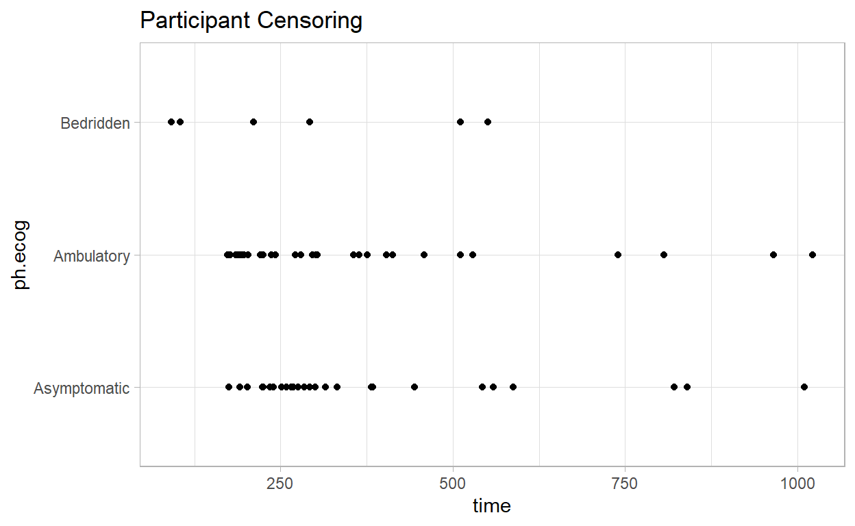

Construct a KM plot to get a feel for the data. The cumulative survival is negatively associated with the ECOG performance score. There is no substantial crossing of the survival curves (that would affect the power of the statistical tests). The curves are similarly shaped. The log-rank test is ideal for similarly shaped distributions and distributions that do not cross. The Breslow, and Tarone-Ware tests are more sensitive alternatives.

km_fit <- survfit(Surv(time, status) ~ ph.ecog, data = cs_dat)

km_fit %>%
  ggsurvplot(
    # data = cs_dat,
    fun = "pct",
    # linetype = "strata", # Change line type by groups
    # pval = TRUE,
    # conf.int = TRUE,
    risk.table = TRUE,
    fontsize = 3, # used in risk table
    surv.median.line = "hv", # median horizontal and vertical ref lines
    ggtheme = theme_light(),
    palette = c("goldenrod", "sienna", "tomato"),
    title = "Kaplan-Meier Survival Function Estimate",
    legend.title = "",
    legend.labs = levels(cs_dat$ph.ecog)
  )

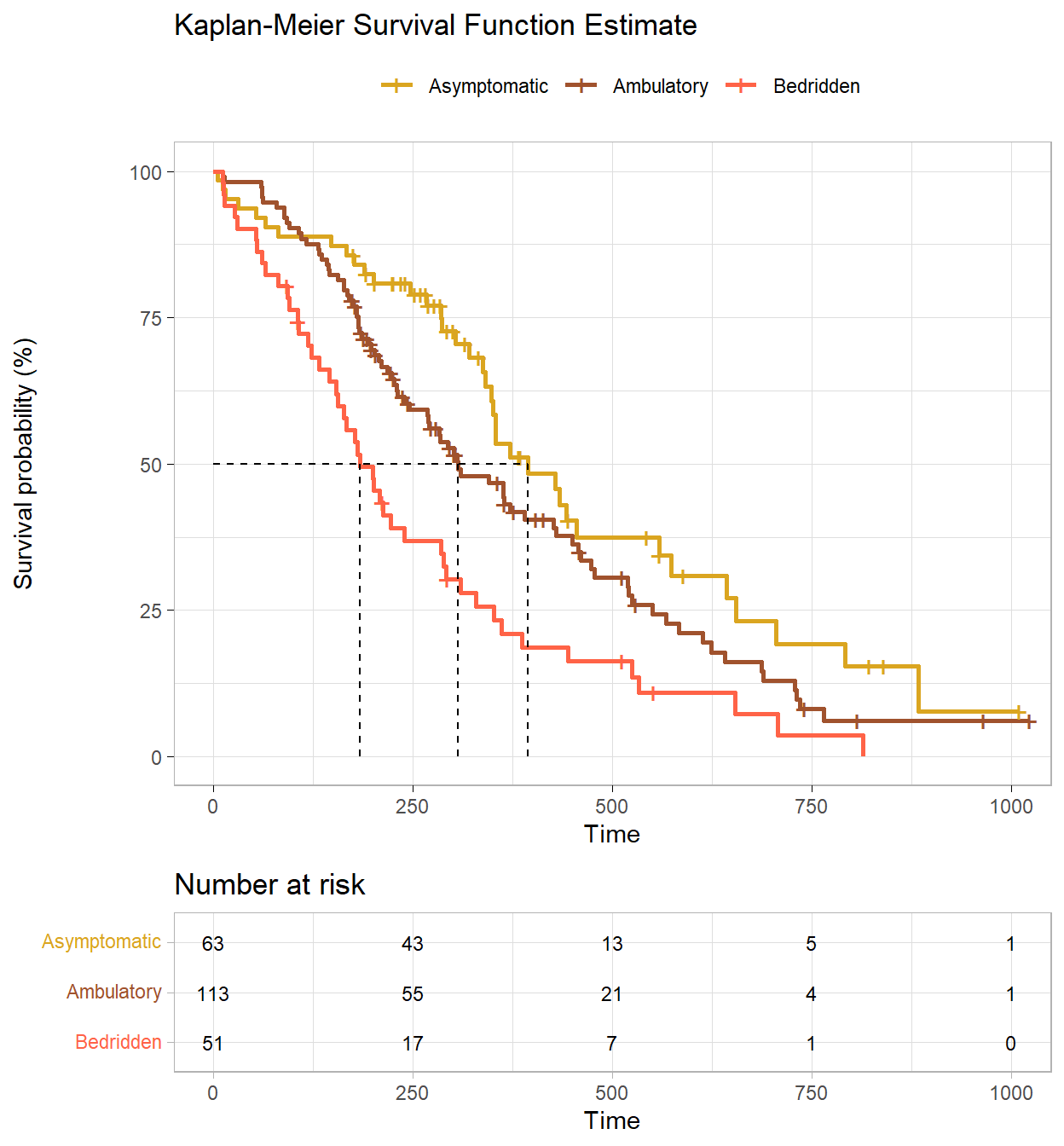
The fitted KM model summary table shows the median survival times.

(km_smry <- summary(km_fit) %>% pluck("table"))

##                      records n.max n.start events    rmean se(rmean) median
## ph.ecog=Asymptomatic      63    63      63     37 465.3131  42.88835    394
## ph.ecog=Ambulatory       113   113     113     82 384.8410  27.28943    306
## ph.ecog=Bedridden         51    51      51     45 255.7636  30.74032    183
##                      0.95LCL 0.95UCL
## ph.ecog=Asymptomatic     348     574
## ph.ecog=Ambulatory       268     429
## ph.ecog=Bedridden        153     288

gtsummary::tbl_survfit(
  list(
    survfit(Surv(time, status) ~ 1, data = cs_dat),
    survfit(Surv(time, status) ~ ph.ecog, data = cs_dat)
    # survfit(Surv(time, status) ~ age, data = cs_dat)
  ),
  probs = 0.5,
  label_header = "**Median Survival**"
) %>%
  gtsummary::add_n() %>%
  gtsummary::add_nevent()

Characteristic	N	Event N	Median Survival
Overall	227	164	310 (285, 363)
ph.ecog	227	164
Asymptomatic			394 (348, 574)
Ambulatory			306 (268, 429)
Bedridden			183 (153, 288)

Participants that were asymptomatic had a median survival time of 394 days (95% CI, 348 to 574 days). This was longer than the ambulatory group, 306 days (95% CI, 268 to 429 days) and bedridden group, 183 days (95% CI, 153 to 288 days).

Determine whether there are significant differences in the fitted survival distributions using a log-rank test (and/or Breslow and Tarone-Ware). If there are differences, run a pairwise comparison post-hoc test to determine which curves differ.

The log-rank test weights the difference at each time point equally. Compared to the other two tests, it places greater emphasis on differences at later rather than earlier time points. The Breslow test (aka generalized Wilcoxon or Gehan) weights the differences by the number at risk at each time point. The effect is to place greater weight on the differences at earlier time points. The Tarone-Ware test weights differences the same way as Breslow, but takes the square root of the number at risk.

(km_diff <- survdiff(Surv(time, status) ~ ph.ecog, data = cs_dat))

## Call:
## survdiff(formula = Surv(time, status) ~ ph.ecog, data = cs_dat)
## 
##                        N Observed Expected (O-E)^2/E (O-E)^2/V
## ph.ecog=Asymptomatic  63       37     54.2    5.4331    8.2119
## ph.ecog=Ambulatory   113       82     83.5    0.0279    0.0573
## ph.ecog=Bedridden     51       45     26.3   13.2582   15.9641
## 
##  Chisq= 19  on 2 degrees of freedom, p= 8e-05

A log rank test was run to determine if there were differences in the survival distribution for the different types of intervention. The survival distributions for the three interventions were statistically significantly different, \(\chi^2\)(2) = 19.0, p < .001.

Breslow and Tarone-Ware are in the coin package.

coin::logrank_test(Surv(time, status) ~ ph.ecog, data = cs_dat, type = "Tarone-Ware")

## 
##  Asymptotic K-Sample Tarone-Ware Test
## 
## data:  Surv(time, status) by
##   ph.ecog (Asymptomatic, Ambulatory, Bedridden)
## chi-squared = 19.009, df = 2, p-value = 7.451e-05

coin::logrank_test(Surv(time, status) ~ ph.ecog, data = cs_dat, type = "Gehan-Breslow")

## 
##  Asymptotic K-Sample Gehan-Breslow Test
## 
## data:  Surv(time, status) by
##   ph.ecog (Asymptomatic, Ambulatory, Bedridden)
## chi-squared = 19.431, df = 2, p-value = 6.034e-05

The log rank test is an ombnibus test. Create a pairwise comparisons table to see which groups differed.

(km_pairwise <- survminer::pairwise_survdiff(Surv(time, status) ~ ph.ecog, data = cs_dat))

## 
##  Pairwise comparisons using Log-Rank test 
## 
## data:  cs_dat and ph.ecog 
## 
##            Asymptomatic Ambulatory
## Ambulatory 0.0630       -         
## Bedridden  9e-05        0.0039    
## 
## P value adjustment method: BH

Adjust the statistical significance to compensate for making multiple comparisons with a Bonferroni correction. There are three comparisons so divide .05 by 3, so the significance is p < .0167.

Pairwise log rank comparisons were conducted to determine which intervention groups had different survival distributions. A Bonferroni correction was made with statistical significance accepted at the p < .017 level. There was a statistically significant difference in survival distributions for the aymptomatic vs bedridden, p < .001, and ambulatory vs bedridden, p = 0.004, groups. However, the survival distributions for the asymptomatic vs ambulatory group were not statistically significant, p = 0.063.

Report the results like this.

227 Men and women diagnosed with advanced lung cancer aged 39 to 82 were monitored up to three years until time of death. Participants were classified into three groups according to their ECOG performance score: asymptomatic (n = 63), symptomatic but completely ambulatory (n = 113), and bedridden at least part of the day (n = 51). A Kaplan-Meier survival analysis (Kaplan & Meier, 1958) was conducted to compare survival times among the three ECOG performance scores. Censored cases were negatively associated with symptom severity, asymptomatic, 26 (41%), symptomatic but completely ambulatory, 31 (27%), and bedridden, 6 (12%) study groups. Participants that were asymptomatic had a median survival time of 394 days (95% CI, 348 to 574 days). This was longer than the ambulatory group, 306 days (95% CI, 268 to 429 days) and bedridden group, 183 days (95% CI, 153 to 288 days). A log rank test was run to determine if there were differences in the survival distribution for the different types of intervention. The survival distributions for the three interventions were statistically significantly different, \(\chi^2\)(2) = 19.0, p < .001. Pairwise log rank comparisons were conducted to determine which intervention groups had different survival distributions. A Bonferroni correction was made with statistical significance accepted at the p < .017 level. There was a statistically significant difference in survival distributions for the aymptomatic vs bedridden, p < .001, and ambulatory vs bedridden, p = 0.004, groups. However, the survival distributions for the asymptomatic vs ambulatory group were not statistically significant, p = 0.063

9.7.2 Cox

The Cox proportional hazards model describes the effect of explanatory variables on survival and can include controlling variables. Add age as a controlling variable.

cox_fit <- coxph(Surv(time, status) ~ ph.ecog + age, data = cs_dat)
(cox_tbl <- cox_fit %>% gtsummary::tbl_regression(exponentiate = TRUE))

Characteristic	HR1	95% CI1	p-value
ph.ecog
Asymptomatic	—	—
Ambulatory	1.43	0.97, 2.11	0.072
Bedridden	2.39	1.52, 3.74	<0.001
age	1.01	0.99, 1.03	0.2
1 HR = Hazard Ratio, CI = Confidence Interval

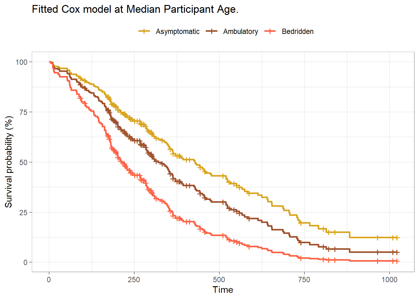
Using a Cox proportional hazards regression analysis, we find the association between ECOG and survival time statistically significant with a Bedridden estimate of 2.39 (95% CI 1.52, 3.74; p<0.001) relative to Asymptomatic. The hazard ratio for Ambulatory was not statistically significant, 1.43 (95% CI 0.97, 2.11; p=0.072).

survfit(cox_fit, newdata = list(ph.ecog = levels(cs_dat$ph.ecog),
                                             age = rep(median(cs_dat$age), 3)), data = cs_dat) %>%
  surv_summary() %>%
  ggsurvplot_df(
    fun = "pct",
    # linetype = "strata", # Change line type by groups
    # conf.int = TRUE,
    surv.median.line = "hv", # median horizontal and vertical ref lines
    ggtheme = theme_light(),
    palette = c("goldenrod", "sienna", "tomato"),
    title = "Fitted Cox model at Median Participant Age.",
    legend.title = "",
    legend.labs = levels(cs_dat$ph.ecog)
  )

9.7.3 Discrete Time

To fit a discrete time model, first create a discrete time data set, on record per relevant time period. You could do this by hand with expand.grid()

cs_glm_dat <- expand.grid(
  time = seq(min(cs_dat$time), max(cs_dat$time), 1),
  patient_id = unique(cs_dat$patient_id)
) %>%
  inner_join(cs_dat, by = "patient_id") %>%
  filter(time.x <= time.y) %>%
  mutate(status = if_else(time.x < time.y, 0, status - 1)) %>%
  rename(time = time.x)

But discSurv::dataLong does this for you.

cs_glm_dat <- cs_dat %>% 
  mutate(status = status - 1) %>%
  discSurv::dataLong("time", "status", timeAsFactor = FALSE)

For example, patient 1 died at time 306, so they have 306 rows in the new data set, with y = 0 for all but the last row.

cs_glm_dat %>% filter(obj == 1) %>% tail()

##       obj timeInt y inst time status age sex    ph.ecog ph.karno pat.karno
## 1.300   1     301 0    3  306      1  74   1 Ambulatory       90       100
## 1.301   1     302 0    3  306      1  74   1 Ambulatory       90       100
## 1.302   1     303 0    3  306      1  74   1 Ambulatory       90       100
## 1.303   1     304 0    3  306      1  74   1 Ambulatory       90       100
## 1.304   1     305 0    3  306      1  74   1 Ambulatory       90       100
## 1.305   1     306 1    3  306      1  74   1 Ambulatory       90       100
##       meal.cal wt.loss patient_id
## 1.300     1175      NA          1
## 1.301     1175      NA          1
## 1.302     1175      NA          1
## 1.303     1175      NA          1
## 1.304     1175      NA          1
## 1.305     1175      NA          1

glm() fits either the log(-log(1-hazard)) or log(hazard / (1-hazard)) as a function of time, controlling for ph.ecog and age. The two links are similar here¹⁴.

cs_glm_dat %>%
  group_by(ph.ecog, timeInt) %>%
  summarise(.groups = "drop", died = sum(y), at_risk = n()) %>%
  mutate(
    hazard = died / at_risk,
    logit_hazard = log(hazard / (1 - hazard)),
    cloglog_hazard = log(-log(1 - hazard))
  ) %>%
  pivot_longer(cols = c(logit_hazard, cloglog_hazard)) %>%
  filter(!hazard %in% c(0, 1)) %>%
  ggplot(aes(x = timeInt, y = value, color = ph.ecog)) +
  geom_point() +
  geom_smooth(method = "lm", formula = "y ~ x") +
  facet_wrap(facets = vars(name)) +
  theme_light()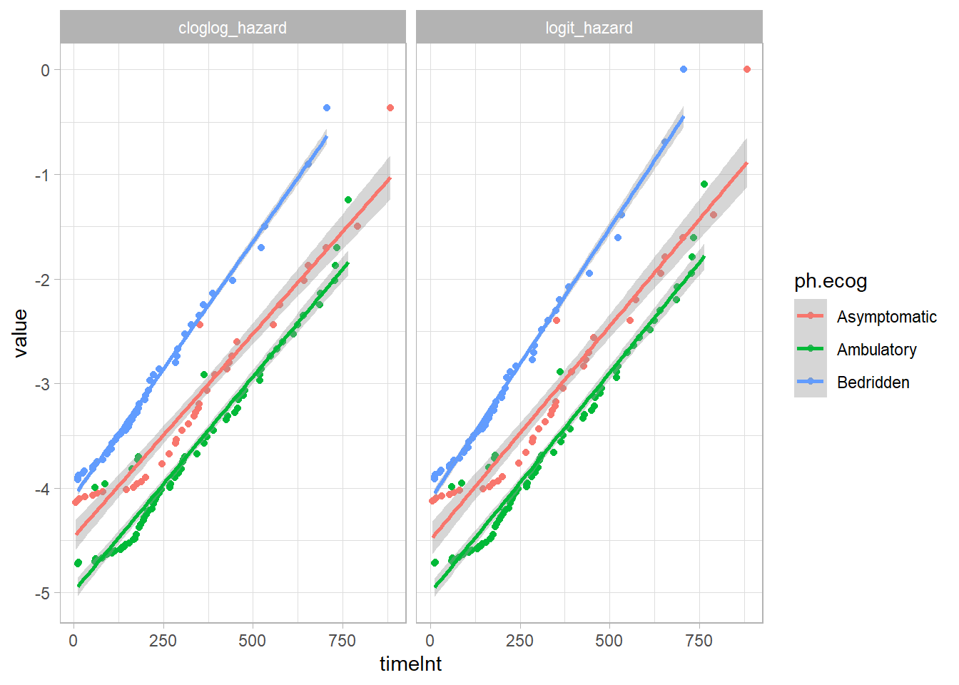

logit_fit <- glm(
  y ~ timeInt + ph.ecog + age, 
  data = cs_glm_dat, 
  family = binomial(link = "logit")
)
(logit_tbl <- logit_fit %>% gtsummary::tbl_regression(exponentiate = TRUE))

Characteristic	OR1	95% CI1	p-value
timeInt	1.00	1.00, 1.00	<0.001
ph.ecog
Asymptomatic	—	—
Ambulatory	1.42	0.97, 2.11	0.081
Bedridden	2.38	1.52, 3.76	<0.001
age	1.01	0.99, 1.03	0.3
1 OR = Odds Ratio, CI = Confidence Interval

Using a discrete time logistic regression analysis with logit link function, we find the association between ECOG and survival time statistically significant with a Bedridden estimate of 2.38 (95% CI 1.52, 3.76; p<0.001) relative to Asymptomatic. The hazard odds ratio for Ambulatory was not statistically significant, 1.42 (95% CI 0.97, 2.11; p=0.081).

cloglog_fit <- glm(
  y ~ timeInt + ph.ecog + age, 
  data = cs_glm_dat, 
  family = binomial(link = "cloglog")
)
(cloglog_tbl <- cloglog_fit %>% gtsummary::tbl_regression(exponentiate = TRUE))

Characteristic	HR1	95% CI1	p-value
timeInt	1.00	1.00, 1.00	<0.001
ph.ecog
Asymptomatic	—	—
Ambulatory	1.41	0.97, 2.11	0.081
Bedridden	2.38	1.52, 3.75	<0.001
age	1.01	0.99, 1.03	0.3
1 HR = Hazard Ratio, CI = Confidence Interval

Using a discrete time logistic regression analysis with complementary log-log link function, we find the association between ECOG and survival time statistically significant with a Bedridden estimate of 2.38 (95% CI 1.52, 3.75; p<0.001) relative to Asymptomatic. The hazard ratio for Ambulatory was not statistically significant, 1.41 (95% CI 0.97, 2.11; p=0.081).

9.7.4 Reporting

The reporting below uses the Cox model rather than the discrete time model.

Participants were randomly assigned to three different interventions in order to quit smoking: a hypnotherapy programme (n = 50), wearing nicotine patches (n = 50) and using e-cigarettes (n = 50). Kaplan-Meier survival analysis (Kaplan & Meier, 1958) was conducted to compare the three different interventions for their effectiveness in preventing smoking resumption. A similar percentage of censored cases was present in the hypnotherapy (12.0%), nicotine patch (14.0%) and e-cigarette (14.0%) intervention groups and the pattern of censoring was similar. Participants that underwent the hypnotherapy programme had a median time to smoking resumption of 69.0 (95% CI, 45.2 to 92.8) days. This was longer than the groups receiving nicotine patches or e-cigarettes, which had identical median times to smoking resumption of 9.0 (95% CI, 6.6 to 11.4) days and 9.0 (95% CI, 7.1 to 10.9) days, respectively. A log rank test was conducted to determine if there were differences in the survival distributions for the different types of intervention. The survival distributions for the three interventions were statistically significantly different, χ2(2) = 25.818, p < .0005. Pairwise log rank comparisons were conducted to determine which intervention groups had different survival distributions. A Bonferroni correction was made with statistical significance accepted at the p < .0167 level. There was a statistically significant difference in survival distributions for the hypnotherapy vs nicotine patch intervention, χ2(1) = 11.035, p = .001, and hypnotherapy vs e-cigarette intervention, χ2(1) = 29.003, p < .0005. However, the survival distributions for the e-cigarette and nicotine patch interventions were not statistically significantly different, χ2(1) = 1.541, p = .214.

References

Laerd. 2015. Statistical Tutorials and Software Guides. https://statistics.laerd.com/.

Moore, Dirk F. 2016. Applied Survival Analysis Using r. 1st ed. New York, NY: Springer. https://eohsi.rutgers.edu/eohsi-directory/name/dirk-moore/.

---

11. See neat discussion in Note section of Surv() help file.↩︎

12. https://www.ncbi.nlm.nih.gov/pmc/articles/PMC5233524/?msclkid=2bbc1508ac1f11ecad286fc872ce9a29↩︎

13. This formulation is derived from the relationship between the survival function to a baseline survival, \(S(t) = S_0(t)^\exp{Xb}\). See German Rodriguez’s course notes.↩︎

14. Full discussion on Rens van de Schoot.↩︎