Chapter 6 Sentiment Analysis
6.1 What is sentiment analysis?
Sentiment analysis is a method of determining the emotional content of a text, a method that is useful and accurate in all cases, and has no underlying problems whatsoever. We can of course rely on sentiment analysis to transform the emotion of a text into a scale of -1 to 1, and this doesn’t oversimplify the complexity of human emotion at all. New methods of sentiment analysis are being developed all the time, and these new methods are so much better than the old ones, and are not just a rebranding of the same solutions that have been around since the 80s.
sentiment_score: 1.0, very positive!6.2 Where is sentiment analysis used?
More places than you think! This text analysis technique has found its way into innumerable social science papers, global stock market predictions, and even content moderation.
We’ll do a basic example today, looking at the sentiment of each chapter of a book of your choice.
6.3 Classwork: Find a text
In our example case, we’ll be using the original German edition of Herman Hesse’s Siddartha, which is available on Project Gutenberg. Feel free to download a book in a language of your choice, or a (long) text from anywhere you like.
We’ll first load the article and split it into separate lines.
When you load some files, you’ll see that \n is the line separator
(usually found on files created on Mac or Linux), and some use the \r\n separator,
which is usually found on files created on Windows.
It’s essentially the same thing, and here we split by \r\n to get the lines of the text.
str_split_1() is a function from the stringr package, which splits a string into a vector of strings.
str_split() also exists, but it returns a list of vectors, which is not what we want here.
We then rename the one column that we get to text, for clarity.
Some of the text downloaded from Gutenberg isn’t really useful for us, with some information at the beginning and some copyright stuff at the end.
We can eliminate those with head() and tail(), which return the first and last n rows of a data frame, respectively.
A useful little trick is that tail() with a negative number returns all but the first n rows of a vector or data frame, like so:
## [1] 3 4 5 6 7 8 9 10 11 12Then, to eliminate the first 61 lines from the beginning, and only keep until line 3930 (for this specific book, of course), we can do the following:
Our next task is to filter out all the blank lines that don’t contain any information. These don’t really contain any information, so we can just drop them.
## # A tibble: 3,351 × 1
##    text
##    <chr>
##  1 DER SOHN DES BRAHMANEN
##  2 Im Schatten des Hauses, in der Sonne des Flußufers bei den Booten, im Schatt…
##  3 des Salwaldes, im Schatten des Feigenbaumes wuchs Siddhartha auf, der
##  4 schöne Sohn des Brahmanen, der junge Falke, zusammen mit Govinda, seinem Fre…
##  5 Brahmanensohn.  Sonne bräunte seine lichten Schultern am Flußufer,
##  6 beim Bade, bei den heiligen Waschungen, bei den heiligen Opfern.
##  7 Schatten floß in seine schwarzen Augen im Mangohain, bei den
##  8 Knabenspielen, beim Gesang der Mutter, bei den heiligen Opfern, bei
##  9 den Lehren seines Vaters, des Gelehrten, beim Gespräch der Weisen.
## 10 Lange schon nahm Siddhartha am Gespräch der Weisen teil, übte sich mit
## # ℹ 3,341 more rows
Next, let’s add line numbers to our data frame. Each row is a line of text,
so we can just use dplyr’s row_number() to get the line number.
Next, we need to add chapter numbers. This will be a bit weird. Looking through the text, we can see that the chapter titles are all in all-caps.
We can then assume that everything that is in all caps is a chapter title (well, probably).
We can check this in R by checking if the title is in all caps. R, confusingly, does not have a
is_upper() function like most languages, so we can only check if it is upper case by comparing
it to
## # A tibble: 3,351 × 3
##    text                                           line_number is_chapter_heading
##    <chr>                                                <int> <lgl>
##  1 DER SOHN DES BRAHMANEN                                   1 TRUE
##  2 Im Schatten des Hauses, in der Sonne des Fluß…           2 FALSE
##  3 des Salwaldes, im Schatten des Feigenbaumes w…           3 FALSE
##  4 schöne Sohn des Brahmanen, der junge Falke, z…           4 FALSE
##  5 Brahmanensohn.  Sonne bräunte seine lichten S…           5 FALSE
##  6 beim Bade, bei den heiligen Waschungen, bei d…           6 FALSE
##  7 Schatten floß in seine schwarzen Augen im Man…           7 FALSE
##  8 Knabenspielen, beim Gesang der Mutter, bei de…           8 FALSE
##  9 den Lehren seines Vaters, des Gelehrten, beim…           9 FALSE
## 10 Lange schon nahm Siddhartha am Gespräch der W…          10 FALSE
## # ℹ 3,341 more rows
6.3.1 Cumulative Sums
The next thing we’ll learn is the cumsum() function, short for “cumulative sum”.
A cumulative sum returns a vector the same length as the original, where each element is the sum of all the elements before it. This is sort of like a running total, imagine you’re just counting things as you go along.
For example, if we have the following vector:
Then the cumulative sum would be the total of every number up to that point.
## [1] 10 18 25 31 38 44 536.4 Getting chapter numbers
By running cumsum() on the is_chapter_heading column,
we can get a running total of chapters, which is then our chapter number.
sid <- sid |>
  mutate(is_chapter_heading = text == toupper(text)) |>
  mutate(chapter = cumsum(is_chapter_heading))
## # A tibble: 6 × 3
## line_number is_chapter_heading chapter
## <int> <lgl> <int>
## 1 1 TRUE 1
## 2 2 FALSE 1
## 3 3 FALSE 1
## 4 4 FALSE 1
## 5 5 FALSE 1
## 6 6 FALSE 1We can then separate the chapter headings out into their own dataframe, which we can re-connect later:
chapter_titles <- sid |>
  filter(is_chapter_heading) |>
  distinct(text, chapter) |>
  rename(chapter_title = text)

chapter_titles
## # A tibble: 12 × 2
## chapter_title chapter
## <chr> <int>
## 1 DER SOHN DES BRAHMANEN 1
## 2 BEI DEN SAMANAS 2
## 3 GOTAMA 3
## 4 ERWACHEN 4
## 5 KAMALA 5
## 6 BEI DEN KINDERMENSCHEN 6
## 7 SANSARA 7
## 8 AM FLUSSE 8
## 9 DER FÄHRMANN 9
## 10 DER SOHN 10
## 11 OM 11
## 12 GOVINDA 12Now, with the data clean, we can get to something new!
The next step will be to split the sentences into different words, also removing the punctuation and converting everything to lowercase.
The hard work of doing this has already been done for us, in the tokenizers library.
Unfortunately, it only works with the following languages:
##  [1] "arabic"     "basque"     "catalan"    "danish"     "dutch"
##  [6] "english"    "finnish"    "french"     "german"     "greek"
## [11] "hindi"      "hungarian"  "indonesian" "irish"      "italian"
## [16] "lithuanian" "nepali"     "norwegian"  "porter"     "portuguese"
## [21] "romanian"   "russian"    "spanish"    "swedish"    "tamil"
## [26] "turkish"
If you’re using something besides these, you might have to search around for a tokenizer that will work with your language, or build one yourself.
But what does a tokenizer do? Let’s take a look at a simple example:
tokenize_word_stems(
  "Hast du etwas Zeit für mich?
  Dann singe ich ein Lied für dich
  Von 99 Luftballons",
  language = "german"
)
## [[1]]
## [1] "hast" "du" "etwas" "zeit" "fur"
## [6] "mich" "dann" "sing" "ich" "ein"
## [11] "lied" "fur" "dich" "von" "99"
## [16] "luftballon"Here, we can see that the tokenizer has split the text into individual words, and also stemmed the words, removing the suffixes and prefixes to get the root of the word. This will make things easier to match things like “sing” and “singing” together, as they both have the same root.
We can then use this tokenizer to split the text into words,
and then unnest the words into their own rows using unnest().
sid <- sid |>
  mutate(word = tokenize_word_stems(text, language = "german")) |>
  unnest(word) |>
  select(-text)
sid
## # A tibble: 34,409 × 4
## line_number is_chapter_heading chapter word
## <int> <lgl> <int> <chr>
## 1 1 TRUE 1 der
## 2 1 TRUE 1 sohn
## 3 1 TRUE 1 des
## 4 1 TRUE 1 brahman
## 5 2 FALSE 1 im
## 6 2 FALSE 1 schatt
## 7 2 FALSE 1 des
## 8 2 FALSE 1 haus
## 9 2 FALSE 1 in
## 10 2 FALSE 1 der
## # ℹ 34,399 more rows6.5 Special Case: Languages without spaces
Some languages, such as Chinese, Thai and ancient Greek do not use spaces between words. We can see that this passage, (The first sentence from the book To Live by Yu Hua, which I highly recommend) contains punctuation, but no spaces.
This makes it difficult to tokenize the text, and we have to rely on other methods to split the text into words. This is very language-specific, and an imperfect science, but for most languages t0here are good tools available.
Going character-by-character would be nonsensical; 快樂, meaning happy, would definitely be a positive word, but 快 and 樂 separately could9 be interpreted as “fast music”, probably neutral.
##  [1] "我" "比" "現" "在" "年" "輕" "十" "歲" "的" "時" "候" "," "獲" "得" "了"
## [16] "一" "個" "遊" "手" "好" "閒" "的" "職" "業" "," "去" "鄉" "間" "收" "集"
## [31] "民" "間" "歌" "謠" "。"
Instead, we could use the package jiebaR to split the passage into much more meaningful words:
## Loading required package: jiebaRD## [1] "我" "比" "現在" "年輕" "十歲" "的"
## [7] "時候" "獲得" "了" "一個" "遊手好閒" "的"
## [13] "職業" "去" "鄉間" "收集" "民間" "歌謠"Much better!
6.6 Calculating sentiment
6.6.1 An important part of learning anything in the 2020s is learning how to find stuff yourself,
Which you’ll probably have to do to to find a “sentiment analysis dictionary.”, the last piece of today’s puzzle.
For our German text, I found a sentiment dictionary from the University of Leipzig (https://wortschatz.uni-leipzig.de/de),
but you’ll need to work this out yourself.
6.7 Class work: Donwloading a sentiment dictionary
Find a sentiment dictionary online, download it, load it into R, and clean the data. The results should look something like this:
download.file("https://downloads.wortschatz-leipzig.de/etc/SentiWS/SentiWS_v2.0.zip", "sentiws.zip")
unzip("sentiws.zip")
positive_words <- read_delim("SentiWS_v2.0_Positive.txt", delim = "\t", col_names = FALSE, show_col_types = FALSE)
negative_words <- read_delim("SentiWS_v2.0_Negative.txt", delim = "\t", col_names = FALSE, show_col_types = FALSE)
sentiment_df <- rbind(
positive_words,
negative_words
)
colnames(sentiment_df) <- c("word", "sentiment", "delete_me")
sentiment_df <- sentiment_df |>
select(-delete_me) |>
mutate(word = str_replace(word, "\\|NN", "")) |>
mutate(word = tolower(word)) |>
mutate(word = str_replace_all(word, "\\|adjx", "")) |>
mutate(word = str_replace_all(word, "\\|vvinf", "")) |>
arrange(word)
sentiment_df## # A tibble: 3,471 × 2
## word sentiment
## <chr> <dbl>
## 1 abbau -0.058
## 2 abbauen -0.0578
## 3 abbrechen -0.348
## 4 abbruch -0.0048
## 5 abdanken -0.0048
## 6 abdankung -0.0048
## 7 abdämpfen -0.0048
## 8 abdämpfung -0.0048
## 9 abfall -0.0048
## 10 abfallen -0.0048
## # ℹ 3,461 more rowsThe sentiment dictonary can come in a number of different forms; some having a single score for each word, some having multiple scores for each word (for one of several emotions, for example).
6.8 Joins
We have all the parts we need, and our final step is to join them together. For this, we have to touch on an important concept in databases, the join.
A join is just a way of combining two data frames together, based on a common column.
For example, let’s say we have two data frames, one with the names of people and their jobs, and one with their ages:
jobs <- data.frame(
  person = c("Billy", "Bob", "Sue"),
  job = c("Computational Social Scientist", "Fighter Pilot", "Pig Farmer")
)
jobs
## person job
## 1 Billy Computational Social Scientist
## 2 Bob Fighter Pilot
## 3 Sue Pig Farmer## person age
## 1 Sue 55
## 2 Billy 68
## 3 Jim 22Some of the data in these doesn’t match up, and some of the data is missing. That’s no big deal, we can still join them together in four different ways.
6.8.1 Inner Join
An inner_join() will only keep the rows that match in both data frames.
## Joining with `by = join_by(person)`## person job age
## 1 Billy Computational Social Scientist 68
## 2 Sue Pig Farmer 556.8.2 Left Join
A left_join() will keep all the rows in the first data frame, and only the rows in the second data frame that match.
## Joining with `by = join_by(person)`## person job age
## 1 Billy Computational Social Scientist 68
## 2 Bob Fighter Pilot NA
## 3 Sue Pig Farmer 556.8.3 Right Join
A right_join() will keep all the rows in the second data frame, and only the rows in the first data frame that match.
## Joining with `by = join_by(person)`## person job age
## 1 Billy Computational Social Scientist 68
## 2 Sue Pig Farmer 55
## 3 Jim <NA> 226.9 Calculating sentiment
Now, assuming that:
- the column names are the same
- some of the values overlap
We can join two data frames together, using left_join().
In my experience, 99% of the time that we’re joining dataframes, we’ll want to use a left join.
## Joining with `by = join_by(word)`## Warning in left_join(sid, sentiment_df): Detected an unexpected many-to-many relationship between `x` and `y`.
## ℹ Row 3243 of `x` matches multiple rows in `y`.
## ℹ Row 1378 of `y` matches multiple rows in `x`.
## ℹ If a many-to-many relationship is expected, set `relationship = "many-to-many"` to silence
## this warning.## # A tibble: 34,431 × 5
## line_number is_chapter_heading chapter word sentiment
## <int> <lgl> <int> <chr> <dbl>
## 1 1 TRUE 1 der 0
## 2 1 TRUE 1 sohn 0
## 3 1 TRUE 1 des 0
## 4 1 TRUE 1 brahman 0
## 5 2 FALSE 1 im 0
## 6 2 FALSE 1 schatt 0
## 7 2 FALSE 1 des 0
## 8 2 FALSE 1 haus 0
## 9 2 FALSE 1 in 0
## 10 2 FALSE 1 der 0
## # ℹ 34,421 more rowsThis gives us the sentiment of each word, using the sentiment dictionary we found earlier.
While we’re at it, let’s also join in the chapter titles.
## Joining with `by = join_by(chapter)`## # A tibble: 34,431 × 6
## line_number is_chapter_heading chapter word sentiment chapter_title
## <int> <lgl> <int> <chr> <dbl> <chr>
## 1 1 TRUE 1 der 0 DER SOHN DES BRAHMA…
## 2 1 TRUE 1 sohn 0 DER SOHN DES BRAHMA…
## 3 1 TRUE 1 des 0 DER SOHN DES BRAHMA…
## 4 1 TRUE 1 brahman 0 DER SOHN DES BRAHMA…
## 5 2 FALSE 1 im 0 DER SOHN DES BRAHMA…
## 6 2 FALSE 1 schatt 0 DER SOHN DES BRAHMA…
## 7 2 FALSE 1 des 0 DER SOHN DES BRAHMA…
## 8 2 FALSE 1 haus 0 DER SOHN DES BRAHMA…
## 9 2 FALSE 1 in 0 DER SOHN DES BRAHMA…
## 10 2 FALSE 1 der 0 DER SOHN DES BRAHMA…
## # ℹ 34,421 more rowsNow, as we learned earlier, we can use group_by() and summarise() to get the average sentiment of each chapter.
sid |>

  group_by(chapter, chapter_title) |>
  summarise(sentiment = mean(sentiment), words = max(row_number()))
## `summarise()` has grouped output by 'chapter'. You can override using the
## `.groups` argument.## # A tibble: 12 × 4
## # Groups: chapter [12]
## chapter chapter_title sentiment words
## <int> <chr> <dbl> <int>
## 1 1 DER SOHN DES BRAHMANEN -0.000367 2347
## 2 2 BEI DEN SAMANAS -0.00219 2890
## 3 3 GOTAMA -0.000712 2753
## 4 4 ERWACHEN -0.00323 1325
## 5 5 KAMALA 0.00176 4054
## 6 6 BEI DEN KINDERMENSCHEN -0.000603 2615
## 7 7 SANSARA -0.00499 2781
## 8 8 AM FLUSSE -0.0000729 3625
## 9 9 DER FÄHRMANN 0.000663 3745
## 10 10 DER SOHN -0.000927 2826
## 11 11 OM -0.00323 2057
## 12 12 GOVINDA 0.00195 3413We now have the average sentiment for each chapter of the book!
From this, we can see that Kamala and Der Fährman are the only positive chapters, with the rest in the negative. Let’s plot it with ggplot()
sid |>
  group_by(chapter) |>
  summarise(sentiment = mean(sentiment), words = max(row_number())) |>
  ggplot() +
  geom_col(aes(x = chapter, y = sentiment)) +
  lims(y = c(-0.01, 0.01))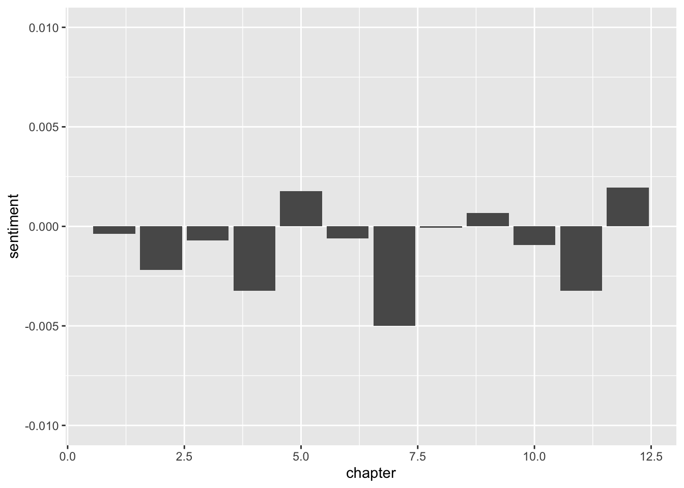
Again, this is the simplest possible way of doing things, but by doing it manually, you’re already way ahead of most social scientists in terms of sentiment analysis.
There have been some really great innovations using deep learning and neural networks to do sentiment analysis, but these are often black boxes, but these are essentially black boxed ways of accomplishing the same thing.
But how do we know this is correct? We would simply have to manually validate it, which will be the topic of next week’s lecture.
Kind of, not really. Please give me a better example↩︎