Chapter 5 Scraping the Web II: Reading HTML
5.1 Making fake news headlines
Fake news is a major problem in our society, and our first task today is to contribute to this problem.
To do this, we’re first going to open out web browsers and go to our favorite news site.
I’m going to use The Associated Press, but you can use any news site you want.
Once you’re there, find a news story you’d like to change the headline of. I’m going to change this article about pandas.
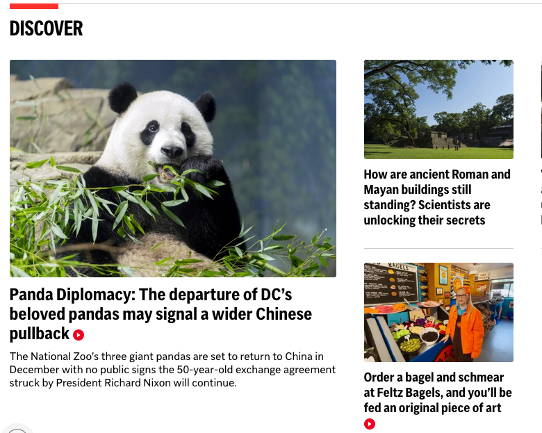
Figure 5.1: The headline we’re going to change.
Now, we’re going to right click on the headline and select Inspect.
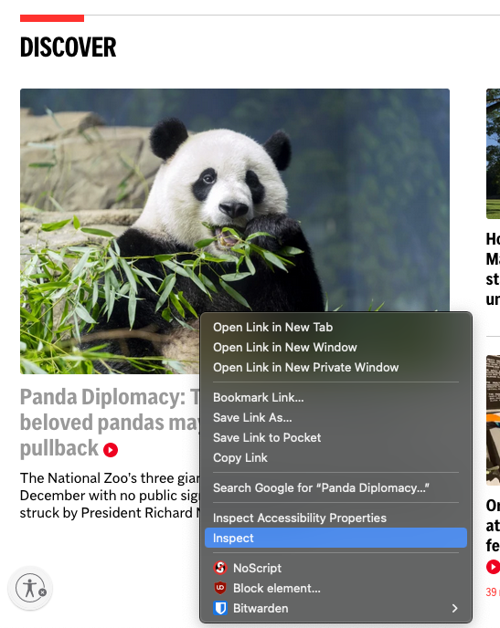
Figure 5.2: It will look slightly different on every browser.
This will bring up the source of the page, which is the HTML code that defines the page. It should be scrolled down to the part of the page that contains the headline.
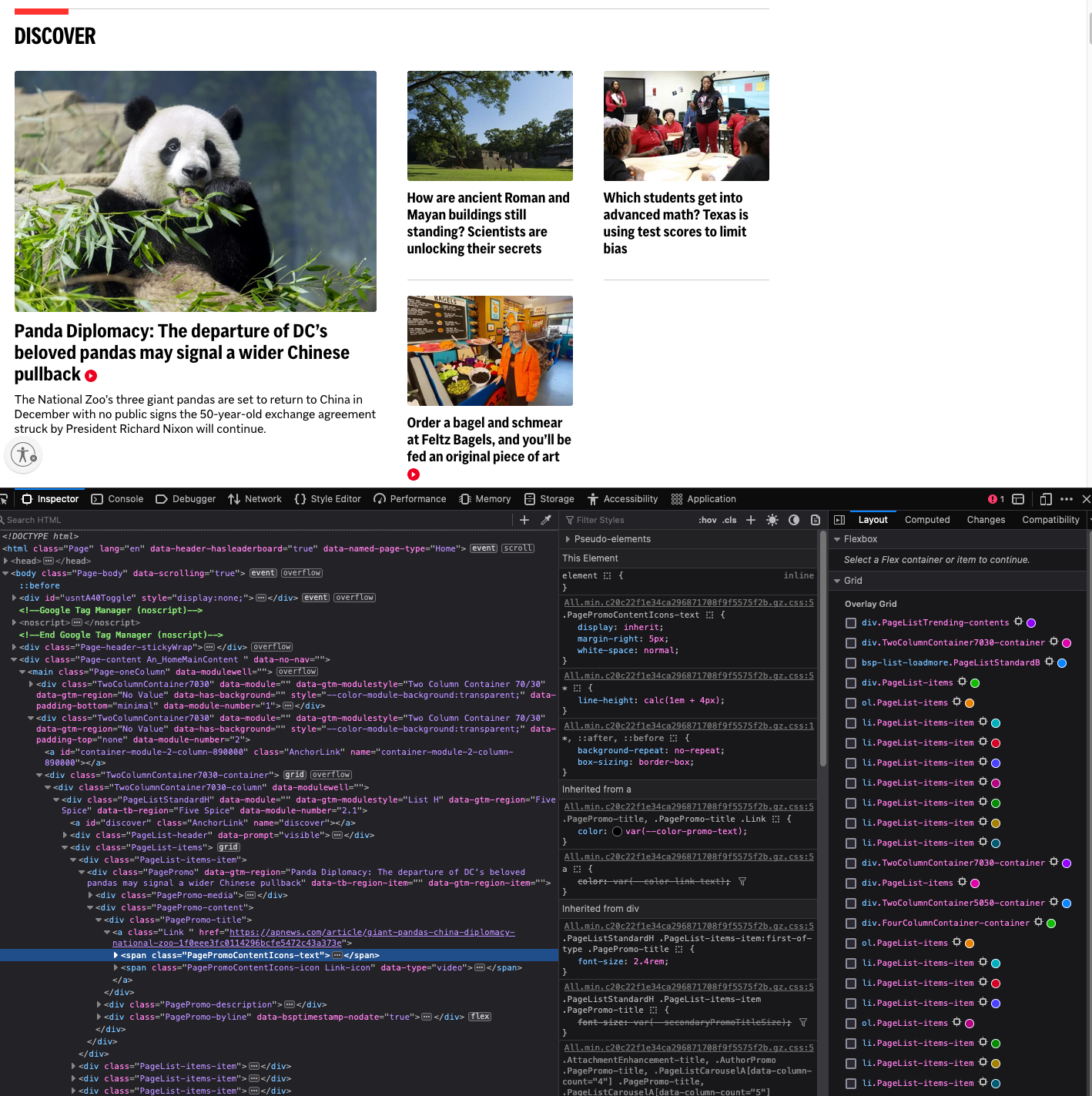
Figure 5.3: HTML files can get pretty big for professional websites.
Now, double click on the headline in the source code. This will allow you to change it to whatever you want.
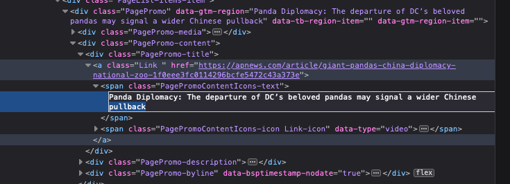
Figure 5.4: Double click on the headline.
Change the headline to whatever you want, and then press enter. You should see the headline change on the page.
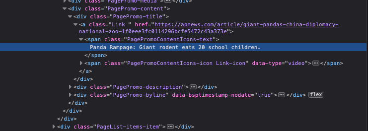
Figure 5.5: Change the headline to whatever you want.
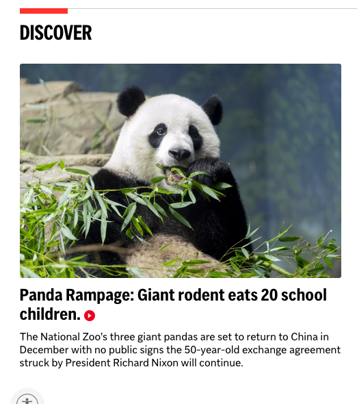
Figure 5.6: Our new headline.
Feel free to screenshot this and share it with your friends, post it on social media, or whatever you want. See how many people you can fool! It’s not morally wrong, because they should have known better than to trust an image on the internet.
5.2 What is HTML?
Hyper Text Markup Language (HTML) is the backbone of the internet; is essentially a text file that defines the structure and content of a web page.
The best way to learn HTML is to look at a simple web page. To start, simply make open the file simple_web_page.html in a text editor (RStudio is fine, but you can use any text editor).
HTML is composed of tags, which are little bits of code enclosed in angle brackets. The most basic tag is the <html> tag, which tells the browser that this is an HTML document.
All HTML documents must have an opening and closing <html> tag.
If you wanted to make a really simple web page, you could Enter the following into your text file:
<html>
Welcome to my web page!
</html>
<html> opens the HTML document, and </html> closes it. Anything between the opening and closing tags is part of the HTML document.
That document would simply produce the following result, if opened in a web page.
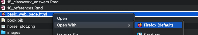
Figure 5.7: This file is now a website.
You should see something like this:
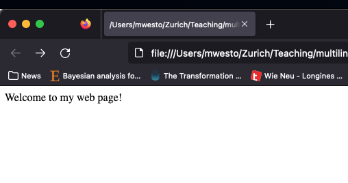
Figure 5.8: The simplest web page you could possibly make.
That’s a good first step, but let’s add a few more things:
5.2.1 Headings
Headings on the page are defined with the <h1> through <h6> tags. <h1> is the largest heading, and <h6> is the smallest. Add a heading to your page by adding the following line between the <html> tags:
<h1>My First Web Page</h1>5.2.2 Paragraphs
Paragraphs are defined with the <p> tag. Add a paragraph to your page by adding the following line between the <html> tags:
<p>This is the first web page I've ever made. I'll cherish it forever.</p>5.2.3 Links
Links are defined with the <a> tag. Add a link to your page by adding the following line between the <html> tags:
<a href="https://learn.shayhowe.com/html-css/">Learn HTML and CSS here.</a>The href attribute tells the browser where to go when the link is clicked. In this case, it’s a link to a website, but it could also be a link to another page on your website.
5.2.4 Head and Body
The <head> tag is used for the parts of the page that aren’t displayed in the browser. This is where you would put things like the title of the page.
The <body> tag is used for the parts of the page that are displayed in the browser. This is where you would put things like headings, paragraphs, links, buttons, etc.
Almost every web page you see looks like this:
<html>
<head>
    <title>Title of the web page</title>
</head>
<body>
  <p>This is the stuff you actually see.
</body>
5.2.5 CSS
CSS (Cascading Style Sheets) is a language that defines the style of an HTML document. It’s what makes web pages look pretty. CSS is a whole other language, so we won’t go into it here, but you can learn more about it here.
A simple example of using CSS might be to change the background and text color of a header. To do this, we would add the following line between the <html> tags:
<style>
h1 {
  background-color: 'red';
  color: 'white';
}
</style>
5.2.6 Classes and ids
CSS is often applied to HTML documents using classes and ids. These are attributes that can be added to HTML tags to tell the browser that they should be styled in a certain way.
For example, if we wanted to change the background color of only one paragraph, we could add a class to that paragraph, like this:
<p class="special">90s kids remember making our own MySpace CSS themes.</p>Then, we could add the following CSS to our page:
<style>
.special {
  background-color: 'blue';
  color: 'yellow';
}
</style>
This would change the background color of only the paragraph with the class special.
5.2.7 Divs
Another way to apply CSS to HTML documents is to use divs. Divs are defined with the <div> tag, and they are used to group together other HTML elements. For example, we could group together all of the paragraphs on our page like this:
<div class="main-content">
  <p>This is the first web page I've ever made. I'll cherish it forever.</p>
  <p class="special">90s kids remember making our own MySpace CSS themes.</p>
  <p>My favorite color is green.</p>
</div>
Then, we could add the following CSS to our page:
<style>
.main-content {
  background-color: 'green';
  color: 'yellow';
}
</style>
This would change the background color of all of the paragraphs in the main-content div,
but not the paragraph with the class special, because the special paragraph
is a child of the main-content div.
5.2.8 Our final web page
Here’s what our final web page looks like:
<html>

<head>
    <title>My First Web Page</title>
    <style>
        h1 {
            background-color: red;
            color: white;
        }

        .special {
            background-color: blue;
            color: yellow;
        }

        .main-content {
            background-color: green;
            color: yellow;
        }
    </style>
</head>

<body>
    <h1>My First Web Page</h1>
    <div class="main-content">
        <p>This is the first web page I've ever made. I'll cherish it forever.</p>
        <p class="special">90s kids remember making our own MySpace CSS themes.</p>
        <p>My favorite color is green.</p>
    </div>
    <a href="https://learn.shayhowe.com/html-css/">Learn HTML and CSS here.</a>
</body>

</html>
5.2.9 Don’t do this.
This is not a web design class. I’m only teaching you this so that you learn how to read it. There’s so much more you need know to make a good web page.
However, web design is really cool, and it’s something you could learn on your own if you wanted to.
I recommend the following resources to get started:
5.3 Reading HTML in R.
The reason you learned this is to learn how to read html, which is essential for being able to extract data from your web page.
Let’s start by taking a look at the previous chapter. We can first download it,
using our friend the download.file() function.
Now, you should have chapter 5 in your file folder. To read this, we’ll use the library rvest
##
## Attaching package: 'rvest'
## The following object is masked from 'package:readr':
##
## guess_encodingFollowing the same pattern as opening other file types, we can now open this with read_html()
We can then pipe it into the function html_elements() This can take a n element, like h2 or a, a class like .special, or an id like #number-5
## {xml_nodeset (12)}
##  [1] <h2>\n<span class="header-section-number">3.1</span> Downloading data<a  ...
##  [2] <h2>\n<span class="header-section-number">3.2</span> CSV<a href="data-fo ...
##  [3] <h2>\n<span class="header-section-number">3.3</span> Pivoting data<a hre ...
##  [4] <h2>\n<span class="header-section-number">3.4</span> Renaming columns.<a ...
##  [5] <h2>\n<span class="header-section-number">3.5</span> Math on columns.<a  ...
##  [6] <h2>\n<span class="header-section-number">3.6</span> Sorting<a href="dat ...
##  [7] <h2>\n<span class="header-section-number">3.7</span> Class Work: Getting ...
##  [8] <h2>\n<span class="header-section-number">3.8</span> JSON<a href="data-f ...
##  [9] <h2>\n<span class="header-section-number">3.9</span> Group_by and Summar ...
## [10] <h2>\n<span class="header-section-number">3.10</span> Class work: Groupi ...
## [11] <h2>\n<span class="header-section-number">3.11</span> XLSX<a href="data- ...
## [12] <h2>\n<span class="header-section-number">3.12</span> Class work: Diggin ...## {xml_nodeset (13)}
## [1] <span class="header-section-number">Chapter 3</span>
## [2] <span class="header-section-number">3.1</span>
## [3] <span class="header-section-number">3.2</span>
## [4] <span class="header-section-number">3.3</span>
## [5] <span class="header-section-number">3.4</span>
## [6] <span class="header-section-number">3.5</span>
## [7] <span class="header-section-number">3.6</span>
## [8] <span class="header-section-number">3.7</span>
## [9] <span class="header-section-number">3.8</span>
## [10] <span class="header-section-number">3.9</span>
## [11] <span class="header-section-number">3.10</span>
## [12] <span class="header-section-number">3.11</span>
## [13] <span class="header-section-number">3.12</span>But, we can see that there’s a problem; it still has lots of HTML dirtying the thing up. To solve this, we want to just extract the text from the html, by using the html_text() function.
##  [1] "3.1 Downloading data"
##  [2] "3.2 CSV"
##  [3] "3.3 Pivoting data"
##  [4] "3.4 Renaming columns."
##  [5] "3.5 Math on columns."
##  [6] "3.6 Sorting"
##  [7] "3.7 Class Work: Getting data from a data frame"
##  [8] "3.8 JSON"
##  [9] "3.9 Group_by and Summarize"
## [10] "3.10 Class work: Grouping and summarizing"
## [11] "3.11 XLSX"
## [12] "3.12 Class work: Digging thorugh data"
html_elements() selects everything that has that element, ID, or class. The list can get pretty long.
##  [1] "First, we’re going to look at three different common data formats in R.\nYou’ll find these all the time when you search for data online."
##  [2] "Rather than downloading the files manually, we’re going to use R to download\nthem for us. This is a good way to automate the process, and also makes it\neasier to share the code with others."
##  [3] "For this, we’ll use the download.file() function. This takes two arguments:"
##  [4] "Make sure the file type matches the file type you’re downloading. If you’re\ndownloading a .jpg file, the file name should end in .jpg."
##  [5] "For example, if we wanted to download a picture from Wikipedia, we could use:"
##  [6] "First, we’re going to look at a CSV file. CSV stands for “comma-separated values”.\nThese are two-dimensional tables, where each row is a line in the file, and each\ncolumn is separated by a comma. Here’s an example:"
##  [7] "This evaluates to a simple table, like this:"
##  [8] "These are great because you can open them in a text editor and read them,\nand are simple enough to edit. They’re also easy to read into R."
##  [9] "Despite the name, CSV files don’t always use commas to separate the columns.\nSometimes they use semicolons, or tabs, or other characters; the Swiss government really\nlikes semicolons for some reason."
## [10] "Let’s take a look at a real-world example. We’re going to use the Swiss government’s\nBundesamt für Statistik (BFS) website to download some data, about incomes for every\ncommune in Switzerland, originally from here:"
## [11] "https://www.atlas.bfs.admin.ch/maps/13/de/15830_9164_8282_8281/24776.html"
## [12] "We find the download link, and use download.file() to download it:"
## [13] "Once again, let’s take a look at the raw data. Open it in a text editor,\nand it should look something like this:"
## [14] "We can see the following:"
## [15] "In the same way as we did in chapter 3, we can use Import Dataset to import the data into RStudio.\nYou can see complete instructions in the last chapter. The code that we get back should\nlook something like this:"
## [16] "This data has a lot of columns, and isn’t always the easiest to read. One convenient way to glimpse\nat the data is the glimpse() function, which shows us the first few rows of each column:"
## [17] "This flips the data frame on its side, so that the columns are now rows, and the rows are now columns.\nThis makes it easier to see the data types, but is really only useful for taking a peek at our data."
## [18] "For this example, we’ll want the GEO_NAME, VARIABLE, and VALUE columns. We can use the select()\nfunction to select only those columns:"
## [19] "We can now easily look at the data that we’re interested in:"
## [20] "However, we can see this data still has a pretty big problem: the VARIABLE column contains the\nname of the variable, and the VALUE column contains the value of the variable. This means that\nthe VALUE column actually represents two things at the same time: The total income of the\ncommune, and the per-capita income of the commune."
## [21] "We can fix this by using the pivot_wider() function, which takes the values in one column,\nand turns them into columns. We’ll use the VARIABLE column as the column names, and the VALUE\ncolumn as the values. To do this, we’ll use two arguments for pivot_wider(): names_from, which\nis the column that we want to use as the column names, and values_from, which is the column\nthat we want to use as the values."
## [22] "This can be hard to get your brain around, so let’s take a look at the data before and after:"
## [23] "The opposite of pivot_wider() is pivot_longer(), which takes columns and turns them into rows.\nYou can really only understand this from practice, so you’ll get a chance to try it out in your homework."
## [24] "This data is now in the shape we want it, but the column names are still an absolute mess. I really don’t\nwant to type Steuerbares Einkommen pro Einwohner/-in, in Franken every time I want to refer to the\nper-capita income column. We can rename all the columns by just assigning a vector of names to the\ncolnames() function:"
## [25] "Note that if we only wanted to rename one column, it might be easier to use the rename() function:"
## [26] "A little housecleaning: The total income is in millions of francs, so we’ll multiply it by 1,000,000\n4\nto get the actual value. This will save some confusion later on."
## [27] "To change a column, we can just assign a new value to it using mutate():"
## [28] "We can sort the data by using the arrange() function. This takes the column that we want to sort by,\nand the direction that we want to sort in. We can use desc() to sort in descending order, or asc() to\nsort in ascending order. For example, to sort by per-capita income, we can use:"
## [29] "This gives us the 10 communes with the highest per-capita income."
## [30] "Use this data set to answer the following questions:"
## [31] "Our next data format is JSON. JSON stands for “JavaScript Object Notation”, as it was originally\ndesigned to be used in JavaScript. It’s a very flexible format, and is used in pretty much every\nprogramming language."
## [32] "Let’s download and take a look at some JSON, originally from here:"
## [33] "https://data.bs.ch/explore/dataset/100192"
## [34] "This is a list of names given to babies in Basel, by year. We can download it using:"
## [35] "When we look at the raw data, we can see that it’s a list of key-value pairs, where the keys are\nthe column names, and the values are the values. This is a very flexible format, and can be used\nto represent pretty much any data structure. This is a huge dataset"
## [36] "However, R doesn’t really have the ability to read JSON on it’s own, so we’ll need to use a package\nto read it. We’ll use the jsonlite package, which has a function called read_json() that\nreads JSON files into R. Load the library in the usual way:"
## [37] "Now you can use the function read_json() to read the file\n6 into R like so:"
## [38] "As an English-language class, let’s rename the columns to English:"
## [39] "This is a pretty big dataset! We can see the number of rows using the nrow() function:"
## [40] "That’s a lot of babies. But sometimes we need to condense this information into a single number."
## [41] "For this, we can use the group_by() and summarize()\n7\nfunctions. These are a little tricky to\nunderstand, so let’s take a look at an example. Let’s say we want to know how many babies were\nborn in Basel per year. We can use group_by() to group the data by year, and then summarize()\nto summarize the data."
## [42] "We first grouped the data by year, and then summarized the data by summing the total column.\nYou can use quite a few different functions in summarize(), including sum(), mean(), median(),\nmin(), max(), and many more."
## [43] "Let’s say we want to know how many Basel babies have names for each letter of the alphabet."
## [44] "Your resulting table should look like this:"
## [45] "The plot should look like this:\n"
## [46] "Our last data format for the day is XLSX. This is a proprietary format, and is used by Microsoft Excel.\nI’d discourage your form using this unless you have to, but sometimes you’ll find it in the wild,\nand you might have less gifted colleagues who insist on using it."
## [47] ""
## [48] "Let’s download and take a look at some XLSX data, originally from the US Census Bureau:"
## [49] "Normally, I am a big advocate for looking at the plain text of files before you import them, but\nXLSX files are a little different. They’re actually a zip file, with a bunch of XML files inside.\nIf you try to open them in a text editor, you’ll just see a bunch of gibberish."
## [50] ""
## [51] "Of course, you can always open them in Excel, but that’s not very reproducible. Instead, we’ll\nuse the readxl package to read the data into R."
## [52] "Load the library in the usual way:"
## [53] "Now, you can click on your downloaded file in the file editor, and import it just like\nyou did with the CSV file. You can see complete instructions in the last chapter."
## [54] "The code that we get back should look something like this:"
## [55] "Let’s take a look at the data frame we get back:"
## [56] "We have three columns:"
## [57] "First, let’s rename the columns to something a little more sensible:"
## [58] "Next, we can get rid of the blank column. A quick way to do this is to use the select() function\nwith a minus sign in front of the column name that we don’t want:"
## [59] "When we look at the data frame, we can see that the last few rows should be removed,\nbut maybe Puerto Rico should be included in our calculations.\n8"
## [60] "There are a couple ways we could do this, but for now let’s:"
## [61] "First, we use filter() to make a 1-row data frame with just Puerto Rico:"
## [62] "Second, we can use head() to select the first 51 rows of the data frame:"
## [63] "Third, we row-bind the two data frames together:"
## [64] "When we look at the tail of the data frame, we can see that Puerto Rico is now included."
## [65] "Finally, we remove the temporary data frame from memory:"
## [66] "This, if you want, could be plotted like so:"
## [67] ""
## [68] "In groups of 2:"
## [69] "You can type 1e6 instead of 1000000, if you don’t like counting zeros↩︎"
## [70] "Don’t do this in real life, just look up the population↩︎"
## [71] "For now, don’t worry what simplifyVector does.↩︎"
## [72] "R is friendly to both Brits and Americans, so it has both the summarise() and summarize() functions,\nwhich do the exact same thing.↩︎"
## [73] "https://en.wikipedia.org/wiki/Political_status_of_Puerto_Rico↩︎"
Often, getting a list of content isn’t very useful to us, and we can collapse it into
one single string of characters using the paste(collapse=" ") function.
The collapse option is simply what you separate the different string with. For us, a space is fine.
## [1] "First, we’re going to look at three different common data formats in R.\nYou’ll find these all the time when you search for data online. Rather than downloading the files manually, we’re going to use R to download\nthem for us. This is a good way to automate the process, and also makes it\neasier to share the code with others. For this, we’ll use the download.file() function. This takes two arguments: Make sure the file type matches the file type you’re downloading. If you’re\ndownloading a .jpg file, the file name should end in .jpg. For example, if we wanted to download a picture from Wikipedia, we could use: First, we’re going to look at a CSV file. CSV stands for “comma-separated values”.\nThese are two-dimensional tables, where each row is a line in the file, and each\ncolumn is separated by a comma. Here’s an example: This evaluates to a simple table, like this: These are great because you can open them in a text editor and read them,\nand are simple enough to edit. They’re also easy to read into R. Despite the name, CSV files don’t always use commas to separate the columns.\nSometimes they use semicolons, or tabs, or other characters; the Swiss government really\nlikes semicolons for some reason. Let’s take a look at a real-world example. We’re going to use the Swiss government’s\nBundesamt für Statistik (BFS) website to download some data, about incomes for every\ncommune in Switzerland, originally from here: https://www.atlas.bfs.admin.ch/maps/13/de/15830_9164_8282_8281/24776.html We find the download link, and use download.file() to download it: Once again, let’s take a look at the raw data. Open it in a text editor,\nand it should look something like this: We can see the following: In the same way as we did in chapter 3, we can use Import Dataset to import the data into RStudio.\nYou can see complete instructions in the last chapter. The code that we get back should\nlook something like this: This data has a lot of columns, and isn’t always the easiest to read. One convenient way to glimpse\nat the data is the glimpse() function, which shows us the first few rows of each column: This flips the data frame on its side, so that the columns are now rows, and the rows are now columns.\nThis makes it easier to see the data types, but is really only useful for taking a peek at our data. For this example, we’ll want the GEO_NAME, VARIABLE, and VALUE columns. We can use the select()\nfunction to select only those columns: We can now easily look at the data that we’re interested in: However, we can see this data still has a pretty big problem: the VARIABLE column contains the\nname of the variable, and the VALUE column contains the value of the variable. This means that\nthe VALUE column actually represents two things at the same time: The total income of the\ncommune, and the per-capita income of the commune. We can fix this by using the pivot_wider() function, which takes the values in one column,\nand turns them into columns. We’ll use the VARIABLE column as the column names, and the VALUE\ncolumn as the values. To do this, we’ll use two arguments for pivot_wider(): names_from, which\nis the column that we want to use as the column names, and values_from, which is the column\nthat we want to use as the values. This can be hard to get your brain around, so let’s take a look at the data before and after: The opposite of pivot_wider() is pivot_longer(), which takes columns and turns them into rows.\nYou can really only understand this from practice, so you’ll get a chance to try it out in your homework. This data is now in the shape we want it, but the column names are still an absolute mess. I really don’t\nwant to type Steuerbares Einkommen pro Einwohner/-in, in Franken every time I want to refer to the\nper-capita income column. We can rename all the columns by just assigning a vector of names to the\ncolnames() function: Note that if we only wanted to rename one column, it might be easier to use the rename() function: A little housecleaning: The total income is in millions of francs, so we’ll multiply it by 1,000,000\n4\nto get the actual value. This will save some confusion later on. To change a column, we can just assign a new value to it using mutate(): We can sort the data by using the arrange() function. This takes the column that we want to sort by,\nand the direction that we want to sort in. We can use desc() to sort in descending order, or asc() to\nsort in ascending order. For example, to sort by per-capita income, we can use: This gives us the 10 communes with the highest per-capita income. Use this data set to answer the following questions: Our next data format is JSON. JSON stands for “JavaScript Object Notation”, as it was originally\ndesigned to be used in JavaScript. It’s a very flexible format, and is used in pretty much every\nprogramming language. Let’s download and take a look at some JSON, originally from here: https://data.bs.ch/explore/dataset/100192 This is a list of names given to babies in Basel, by year. We can download it using: When we look at the raw data, we can see that it’s a list of key-value pairs, where the keys are\nthe column names, and the values are the values. This is a very flexible format, and can be used\nto represent pretty much any data structure. This is a huge dataset However, R doesn’t really have the ability to read JSON on it’s own, so we’ll need to use a package\nto read it. We’ll use the jsonlite package, which has a function called read_json() that\nreads JSON files into R. Load the library in the usual way: Now you can use the function read_json() to read the file\n6 into R like so: As an English-language class, let’s rename the columns to English: This is a pretty big dataset! We can see the number of rows using the nrow() function: That’s a lot of babies. But sometimes we need to condense this information into a single number. For this, we can use the group_by() and summarize()\n7\nfunctions. These are a little tricky to\nunderstand, so let’s take a look at an example. Let’s say we want to know how many babies were\nborn in Basel per year. We can use group_by() to group the data by year, and then summarize()\nto summarize the data. We first grouped the data by year, and then summarized the data by summing the total column.\nYou can use quite a few different functions in summarize(), including sum(), mean(), median(),\nmin(), max(), and many more. Let’s say we want to know how many Basel babies have names for each letter of the alphabet. Your resulting table should look like this: The plot should look like this:\n Our last data format for the day is XLSX. This is a proprietary format, and is used by Microsoft Excel.\nI’d discourage your form using this unless you have to, but sometimes you’ll find it in the wild,\nand you might have less gifted colleagues who insist on using it. Let’s download and take a look at some XLSX data, originally from the US Census Bureau: Normally, I am a big advocate for looking at the plain text of files before you import them, but\nXLSX files are a little different. They’re actually a zip file, with a bunch of XML files inside.\nIf you try to open them in a text editor, you’ll just see a bunch of gibberish. Of course, you can always open them in Excel, but that’s not very reproducible. Instead, we’ll\nuse the readxl package to read the data into R. Load the library in the usual way: Now, you can click on your downloaded file in the file editor, and import it just like\nyou did with the CSV file. You can see complete instructions in the last chapter. The code that we get back should look something like this: Let’s take a look at the data frame we get back: We have three columns: First, let’s rename the columns to something a little more sensible: Next, we can get rid of the blank column. A quick way to do this is to use the select() function\nwith a minus sign in front of the column name that we don’t want: When we look at the data frame, we can see that the last few rows should be removed,\nbut maybe Puerto Rico should be included in our calculations.\n8 There are a couple ways we could do this, but for now let’s: First, we use filter() to make a 1-row data frame with just Puerto Rico: Second, we can use head() to select the first 51 rows of the data frame: Third, we row-bind the two data frames together: When we look at the tail of the data frame, we can see that Puerto Rico is now included. Finally, we remove the temporary data frame from memory: This, if you want, could be plotted like so: In groups of 2: You can type 1e6 instead of 1000000, if you don’t like counting zeros↩︎ Don’t do this in real life, just look up the population↩︎ For now, don’t worry what simplifyVector does.↩︎ R is friendly to both Brits and Americans, so it has both the summarise() and summarize() functions,\nwhich do the exact same thing.↩︎ https://en.wikipedia.org/wiki/Political_status_of_Puerto_Rico↩︎"there are many other ways to extract data. You can look them up on your own at:
5.4 A sample project: Scraping this book.
We’ll start this assignment by pulling my template project from Github, the same as your homework assignments. The invitation link can be found here:
https://classroom.github.com/a/Usfa2VjF
In this class work, we’ll scrape the website https://www.azlyrics.com
We don’t have a sitemap, so we’ll start by just pulling the band’s page. I’m going to download all the Foo Fighters lyrics, because that’s what I’m listening to as I write this.
First, go to the website and find your favorite band.
Make a folder called lyric_data, and download the page to it.
trying URL 'https://www.azlyrics.com/f/foofighters.html'
downloaded 89 KB
We can then read it into R using read_html()
## {html_document}
## <html lang="en">
## [1] <head>\n<meta http-equiv="Content-Type" content="text/html; charset=UTF-8 ...
## [2] <body class="margin50">\r\n  <nav class="navbar navbar-default navbar-fix ...
Looking at the .html of the page, we can see that all the albums are given the class album,
<div id="6316" class="album">album: <b>"Echoes, Silence, Patience & Grace"</b> (2007)<div>We can select them all using the .album class. Remember that classes are selected with .periods,
ids with #hashtags, and elements with nothing.
##  [1] "album: \"Foo Fighters\" (1995)"
##  [2] "album: \"The Colour And The Shape\" (1997)"
##  [3] "album: \"There Is Nothing Left To Lose\" (1999)"
##  [4] "album: \"One By One\" (2002)"
##  [5] "album: \"In Your Honor\" (2005)"
##  [6] "album: \"Echoes, Silence, Patience & Grace\" (2007)"
##  [7] "album: \"Wasting Light\" (2011)"
##  [8] "compilation: \"Medium Rare\" (2011)"
##  [9] "album: \"Sonic Highways\" (2014)"
## [10] "EP: \"Songs From The Laundry Room\" (2015)"
## [11] "EP: \"Saint Cecilia\" (2015)"
## [12] "album: \"Concrete And Gold\" (2017)"
## [13] "album: \"Medicine At Midnight\" (2021)"
## [14] "soundtrack: \"Dream Widow\" (2022)(as Dream Widow)"
## [15] "album: \"But Here We Are\" (2023)"
## [16] "other songs:"
5.4.1 Getting all links
Now, we want to scrape all the individual posts from this page. We can do this in two steps:
- Find all the links on the first page
- Download all those links
Looking again at the html, we can see that all the songs also have a class associated with them.
<div class="listalbum-item"><a href="/lyrics/foofighters/thepretender.html" target="_blank">The Pretender</a></div>
<div class="listalbum-item"><a href="/lyrics/foofighters/letitdie.html" target="_blank">Let It Die</a></div>
<div class="listalbum-item"><a href="/lyrics/foofighters/erasereplace.html" target="_blank">Erase / Replace</a></div>
<div class="listalbum-item"><a href="/lyrics/foofighters/longroadtoruin.html" target="_blank">Long Road To Ruin</a></div>
Let’s list all those songs, first by selecting the .listalbum-item class,
## {xml_nodeset (198)}
##  [1] <div class="listalbum-item"><a href="/lyrics/foofighters/thisisacall.htm ...
##  [2] <div class="listalbum-item"><a href="/lyrics/foofighters/illstickaround. ...
##  [3] <div class="listalbum-item"><a href="/lyrics/foofighters/bigme13150.html ...
##  [4] <div class="listalbum-item"><a href="/lyrics/foofighters/aloneeasytarget ...
##  [5] <div class="listalbum-item"><a href="/lyrics/foofighters/goodgrief.html" ...
##  [6] <div class="listalbum-item"><a href="/lyrics/foofighters/floaty.html" ta ...
##  [7] <div class="listalbum-item"><a href="/lyrics/foofighters/weeniebeenie.ht ...
##  [8] <div class="listalbum-item"><a href="/lyrics/foofighters/ohgeorge.html"  ...
##  [9] <div class="listalbum-item"><a href="/lyrics/foofighters/forallthecows.h ...
## [10] <div class="listalbum-item"><a href="/lyrics/foofighters/xstatic.html" t ...
## [11] <div class="listalbum-item"><a href="/lyrics/foofighters/wattershed.html ...
## [12] <div class="listalbum-item"><a href="/lyrics/foofighters/exhausted.html" ...
## [13] <div class="listalbum-item">\n<a href="/lyrics/foofighters/winnebago.htm ...
## [14] <div class="listalbum-item">\n<a href="/lyrics/foofighters/podunk.html"  ...
## [15] <div class="listalbum-item">\n<a href="/lyrics/foofighters/howimissyou.h ...
## [16] <div class="listalbum-item">\n<a href="/lyrics/foofighters/ozone.html" t ...
## [17] <div class="listalbum-item"><a href="/lyrics/foofighters/doll.html" targ ...
## [18] <div class="listalbum-item"><a href="/lyrics/foofighters/monkeywrench.ht ...
## [19] <div class="listalbum-item"><a href="/lyrics/foofighters/heyjohnnypark.h ...
## [20] <div class="listalbum-item"><a href="/lyrics/foofighters/mypoorbrain.htm ...
## ...
Then, we select the text inside those elements.
[1] "This Is A Call"
[1] "I'll Stick Around"
[1] "Big Me"
...
...
...
[1] "Wheels"
[1] "Word Forward"
[1] "World (Demo)"
Now, instead of getting the text, we’ll use html_attr() to get a different HTML attribute, the href, which is the link
Now, both of these are pretty useful things, so let’s turn it into a data frame.
Each element them should be a column, so we can just use cbind() to bind the columns.
cbind(
  foo |> html_elements(".listalbum-item") |> html_element("a") |> html_text(),
  foo |> html_elements(".listalbum-item") |> html_element("a") |> html_attr("href")
) |> data.frame()cbind(
foo |> html_elements(".listalbum-item") |> html_element("a") |> html_text(),
foo |> html_elements(".listalbum-item") |> html_element("a") |> html_attr("href")
) |> data.frame() |> head(5) |> knitr::kable()| X1 | X2 |
|---|---|
| This Is A Call | /lyrics/foofighters/thisisacall.html |
| I’ll Stick Around | /lyrics/foofighters/illstickaround.html |
| Big Me | /lyrics/foofighters/bigme13150.html |
| Alone + Easy Target | /lyrics/foofighters/aloneeasytarget13151.html |
| Good Grief | /lyrics/foofighters/goodgrief.html |
This looks good, so let’s save it to a variable.
The default column names are ugly, so let’s give them clearer names:
You can see that the links here are not complete! This is because they are relative links, within the website.
When we try to scrape these, it won’t do anything. We need to add https://www.azlyrics.com to the beginning.
Now, similarly to last week, we should scrape the website, slowly so that we don’t get caught.
This time, let’s do it all in R.
First, we should add a new column called “lyrics”. It should be blank for now.
Once again, we want to use a for loop to go through this new data frame one-by-one.
We take the number of rows in our data frame, and use the index to look at each row one-by-one:
To start, we’ll do this with one row at a time, which we’ll just call row.
I’ll select the 84th row of the data frame:
##            title                                                          link
## 84 The Pretender https://www.azlyrics.com/lyrics/foofighters/thepretender.html
##    lyrics
## 84     NA
We can then access the column of each row using the $ sign, because the columns are where the money is.
We can select the link column:
## [1] "https://www.azlyrics.com/lyrics/foofighters/thepretender.html"Instead of download.file(), we can also load the html directly into memory using read_html()
## {html_document}
## <html lang="en">
## [1] <head>\n<meta http-equiv="Content-Type" content="text/html; charset=UTF-8 ...
## [2] <body class="az-song-text">\r\n  <nav class="navbar navbar-default navbar ...
let’s assign it to a variable:
## {html_document}
## <html lang="en">
## [1] <head>\n<meta http-equiv="Content-Type" content="text/html; charset=UTF-8 ...
## [2] <body class="az-song-text">\r\n  <nav class="navbar navbar-default navbar ...
Looking around the HTML, we see that there’s a class called text-center that contains all the lyrics, as well as some
other stuff. Let’s go ahead and only select that.
## {xml_nodeset (8)}
## [1] <div class="btn-group text-center" role="group">\r\n <a class="btn btn ...
## [2] <div class="top-ad text-center">\r\n <div id="primisPlayer"></ ...
## [3] <div class="text-center noprint">\r\n<!-- Tag ID: azlyrics_atf_leaderboar ...
## [4] <div class="col-lg-2 text-center hidden-md hidden-sm hidden-xs noprint">\ ...
## [5] <div class="col-xs-12 col-lg-8 text-center">\r\n\r\n<div class="div-share ...
## [6] <div class="col-lg-2 text-center hidden-md hidden-sm hidden-xs noprint">\ ...
## [7] <div class="container text-center">\r\n <ul class="nav navbar-na ...
## [8] <div class="container text-center">\r\n <ul class="nav navbar-na ...Everything inside lyrics is just a div, so let’s select all the div nodes, then get the text.
## [1] ""
## [2] "\r \r freestar.config.enabled_slots.push({ placementName: \"azlyrics_atf_leaderboard\", slotId: \"azlyrics_atf_leaderboard\" });\r"
## [3] ""
## [4] "\r\n\r \r \r \r \r \r \r \r \r \r \r \r \r\n\r"
## [5] "\r \r \r \r \r \r \r \r \r \r \r \r \r"
## [6] "\"The Pretender\" lyrics"
## [7] "\r\nFoo Fighters Lyrics\n\r"
## [8] "\r \r"
## [9] "\r Usage of azlyrics.com content by any third-party lyrics provider is prohibited by our licensing agreement. Sorry about that. \r Keep you in the dark\nYou know they all pretend\nKeep you in the dark\nAnd so it all began\n\nSend in your skeletons\nSing as their bones go marching in again\nThey need you buried deep\nThe secrets that you keep are at the ready\nAre you ready?\nI'm finished making sense\nDone pleading ignorance, that whole defense\nSpinning infinity, boy\nThe wheel is spinning me\nIt's never-ending, never-ending\nSame old story\n\nWhat if I say I'm not like the others?\nWhat if I say I'm not just another one of your plays?\nYou're the pretender\nWhat if I say I will never surrender?\nWhat if I say I'm not like the others?\nWhat if I say I'm not just another one of your plays?\nYou're the pretender\nWhat if I say that I'll never surrender?\n\nIn time or so I'm told\nI'm just another soul for sale, oh well\nThe page is out of print\nWe are not permanent, we're\nTemporary, temporary\nSame old story\n\nWhat if I say I'm not like the others?\nWhat if I say I'm not just another one of your plays?\nYou're the pretender\nWhat if I say I will never surrender?\nWhat if I say I'm not like the others?\nWhat if I say I'm not just another one of your plays?\nYou're the pretender\nWhat if I say I will never surrender?\n\nI'm the voice inside your head\nYou refuse to hear\nI'm the face that you have to face\nMirroring your stare\nI'm what's left\nI'm what's right\nI'm the enemy\nI'm the hand that'll take you down\nBring you to your knees\nSo who are you?\nYeah, who are you?\nYeah, who are you?\nYeah, who are you?\n\nKeep you in the dark\nYou know they all pretend\n\nWhat if I say I'm not like the others?\nWhat if I say I'm not just another one of your plays?\nYou're the pretender\nWhat if I say I will never surrender?\nWhat if I say I'm not like the others?\nWhat if I say I'm not just another one of your plays?\nYou're the pretender\nWhat if I say I will never surrender?\n\nWhat if I say I'm not like the others?\n(Keep you in the dark)\nWhat if I say I'm not just another one of your plays?\n(You know they all)\nYou're the pretender\n(Pretend)\nWhat if I say I will never surrender?\nWhat if I say I'm not like the others?\n(Keep you in the dark)\nWhat if I say I'm not just another one of your plays?\n(You know they all)\nYou're the pretender\n(Pretend)\nWhat if I say I will never surrender?\nSo who are you?\nYeah, who are you?\nYeah, who are you?"
## [10] "\r \r if ( /Android|webOS|iPhone|iPod|iPad|BlackBerry|IEMobile|Opera Mini/i.test(navigator.userAgent) ) \r {\r document.getElementById('azmxmbanner').style.display='block';\r document.write('<div style=\"margin-left: auto; margin-right: auto;\">'+\r '<iframe scrolling=\"no\" style=\"border: 0px none; overflow:hidden;\" src=\"//adv.mxmcdn.net/br/t1.0/m_js/e_0/sn_0/l_29710350/su_0/rs_0/tr_3vUCAJUCR58ffwHLbm2upxO0hKUpIuYXaTDIFanVAIXLieRa744L8pxFkSbDaRrQwWGEvCOomrBw4vBknQwR5zVoQW2yV2cGpHkjIRBJaglVn1edaTda17iY9EyIOXOWAUBOusE_wB8FNxpi9qxHibZUNFroGVhuTNxMFO8CarnjDG8LIsrPB9tXSWfRQkXt7madxO0XGSelFIjpYJ44qCMYlmaEWvD8oOcKG2WPPQ08RkDogO-T5wnqHOUCQc18FwxUIiVl0YHBIi5Dc2TldUMn2vIEL32C3Sy9oY5cSEfARzbu_oWpKOhCRzcn1TM_CQ6BQgxCUrL0mFWp1-m0xu81-SPdvoKJA8k4boOwVsaxik7bqdb1Nhj7uGFpy_O6mQ19dxDOp5xU7_BxiCRQSCniGv8Ije7XEiYx9zysIDgI4kSS3jbspevljIEpnQOvc6tF4g/\" width=\"290px\" height=\"50px\"></iframe>'+\r '</div>');\r }\r\n\n"
## [11] "\r Submit Corrections\r"
## [12] "Thanks to yaayaa for adding these lyrics. Thanks to Nour, Jill, jdelmauro7, Nikana for correcting these lyrics."
## [13] "\r \r"
## [14] "Writer(s): Velton Bunch, Gregory Townley\n"
## [15] "The first single from the album. It is one of the band's most successful songs reaching the number 37 on the US Billboard Hot 100."
## [16] "Dave Grohl said about this song, \"A stomping Foo Fighters uptempo song, with a little bit of Chuck Berry in it.\""
## [17] "This song had a working title \"Silver Heart\" and was much slower in tempo. It wasn't planned to be included in the album. Dave Grohl told XFM, \"That song didn't happen until later on in the session. We didn't go into making the record with that song and it happened after we recorded a lot of stuff.\""
## [18] "The song won the Best Hard Rock Performance, and the album won the Best Rock Album awards at the Grammy ceremony in 2008."
## [19] "\r\r\n\r \r freestar.config.enabled_slots.push({ placementName: \"azlyrics_btf_2\", slotId: \"azlyrics_btf_2\" });\r\n\r"
## [20] "\r \r freestar.config.enabled_slots.push({ placementName: \"azlyrics_btf_2\", slotId: \"azlyrics_btf_2\" });\r"
## [21] "\r\nalbum:\"Echoes, Silence, Patience & Grace\"(2007)\n\r\nThe Pretender\nLet It Die\nErase / Replace\nLong Road To Ruin\nCome Alive\nStranger Things Have Happened\nCheer Up, Boys (Your Make-Up Is Running)\nSummer's End\nStatues\nBut, Honestly\nHome\nOnce & For All\n(Japanese Bonus Track)\nSeda\n(Japanese Bonus Track)"
## [22] "album:\"Echoes, Silence, Patience & Grace\"(2007)"
## [23] ""
## [24] "The Pretender"
## [25] "Let It Die"
## [26] "Erase / Replace"
## [27] "Long Road To Ruin"
## [28] "Come Alive"
## [29] "Stranger Things Have Happened"
## [30] "Cheer Up, Boys (Your Make-Up Is Running)"
## [31] "Summer's End"
## [32] "Statues"
## [33] "But, Honestly"
## [34] "Home"
## [35] "Once & For All\n(Japanese Bonus Track)"
## [36] "(Japanese Bonus Track)"
## [37] "Seda\n(Japanese Bonus Track)"
## [38] "(Japanese Bonus Track)"
## [39] "\r\nYou May Also Like\n\r\nLimp Bizkit - \"Rollin' (Air Raid Vehicle)\" Alright, partner, keep on rollin', baby, you know what time it is (Ladies and gentlemen!) (Throw your hands up) (Throw your, your hands up) (Throw your, throw, throw your) (Throw your, your, your...\nSlipknot - \"Duality\" I push my fingers into my eyes It's the only thing that slowly stops the ache But it's made of all the things I have to take Jesus, it never ends, it works its way inside If the pain goes on I have...\nThe Presidents Of The United States Of America - \"Lump\" Lump sat alone in a boggy marsh Totally emotionless except for her heart Mud flowed up into lump's pajamas She totally confused all the passing piranhas She's lump, she's lump She's in my head She's...\nThe Hives - \"Tick Tick Boom\" Alright Två tre, boom! Yeah, I was right all along Yeah, you come taggin' along Exhibit A on a tray, what you say As I throw it in your face? Exhibit B, what you see? Well, that's me I'll put you...\nRed Hot Chili Peppers - \"Don't Forget Me\" I'm an ocean in your bedroom Make you feel warm, make you want to re-assume Now we know it all for sure I'm a dance hall dirty breakbeat Make the snow fall up from underneath your feet Not alone,...\n\r"
## [40] "You May Also Like"
## [41] "Limp Bizkit - \"Rollin' (Air Raid Vehicle)\" Alright, partner, keep on rollin', baby, you know what time it is (Ladies and gentlemen!) (Throw your hands up) (Throw your, your hands up) (Throw your, throw, throw your) (Throw your, your, your..."
## [42] "Slipknot - \"Duality\" I push my fingers into my eyes It's the only thing that slowly stops the ache But it's made of all the things I have to take Jesus, it never ends, it works its way inside If the pain goes on I have..."
## [43] "The Presidents Of The United States Of America - \"Lump\" Lump sat alone in a boggy marsh Totally emotionless except for her heart Mud flowed up into lump's pajamas She totally confused all the passing piranhas She's lump, she's lump She's in my head She's..."
## [44] "The Hives - \"Tick Tick Boom\" Alright Två tre, boom! Yeah, I was right all along Yeah, you come taggin' along Exhibit A on a tray, what you say As I throw it in your face? Exhibit B, what you see? Well, that's me I'll put you..."
## [45] "Red Hot Chili Peppers - \"Don't Forget Me\" I'm an ocean in your bedroom Make you feel warm, make you want to re-assume Now we know it all for sure I'm a dance hall dirty breakbeat Make the snow fall up from underneath your feet Not alone,..."
## [46] "\r \r Search\r \r"
## [47] "\r"
## [48] ""From here, we can use nth() to select one from a vector. It looks like all the lyrics are in no. 9, so let’s select
the 9th node and forget about the rest.
## [1] "\r Usage of azlyrics.com content by any third-party lyrics provider is prohibited by our licensing agreement. Sorry about that. \r Keep you in the dark\nYou know they all pretend\nKeep you in the dark\nAnd so it all began\n\nSend in your skeletons\nSing as their bones go marching in again\nThey need you buried deep\nThe secrets that you keep are at the ready\nAre you ready?\nI'm finished making sense\nDone pleading ignorance, that whole defense\nSpinning infinity, boy\nThe wheel is spinning me\nIt's never-ending, never-ending\nSame old story\n\nWhat if I say I'm not like the others?\nWhat if I say I'm not just another one of your plays?\nYou're the pretender\nWhat if I say I will never surrender?\nWhat if I say I'm not like the others?\nWhat if I say I'm not just another one of your plays?\nYou're the pretender\nWhat if I say that I'll never surrender?\n\nIn time or so I'm told\nI'm just another soul for sale, oh well\nThe page is out of print\nWe are not permanent, we're\nTemporary, temporary\nSame old story\n\nWhat if I say I'm not like the others?\nWhat if I say I'm not just another one of your plays?\nYou're the pretender\nWhat if I say I will never surrender?\nWhat if I say I'm not like the others?\nWhat if I say I'm not just another one of your plays?\nYou're the pretender\nWhat if I say I will never surrender?\n\nI'm the voice inside your head\nYou refuse to hear\nI'm the face that you have to face\nMirroring your stare\nI'm what's left\nI'm what's right\nI'm the enemy\nI'm the hand that'll take you down\nBring you to your knees\nSo who are you?\nYeah, who are you?\nYeah, who are you?\nYeah, who are you?\n\nKeep you in the dark\nYou know they all pretend\n\nWhat if I say I'm not like the others?\nWhat if I say I'm not just another one of your plays?\nYou're the pretender\nWhat if I say I will never surrender?\nWhat if I say I'm not like the others?\nWhat if I say I'm not just another one of your plays?\nYou're the pretender\nWhat if I say I will never surrender?\n\nWhat if I say I'm not like the others?\n(Keep you in the dark)\nWhat if I say I'm not just another one of your plays?\n(You know they all)\nYou're the pretender\n(Pretend)\nWhat if I say I will never surrender?\nWhat if I say I'm not like the others?\n(Keep you in the dark)\nWhat if I say I'm not just another one of your plays?\n(You know they all)\nYou're the pretender\n(Pretend)\nWhat if I say I will never surrender?\nSo who are you?\nYeah, who are you?\nYeah, who are you?"This is better, but it still says “Usage of azlyrics.com content by any third-party lyrics provider is prohibited by our licensing agreement. Sorry about that.” (good thing we didn’t sign an angreement.)
We can get rid of that by using str_replace().
lyrics <- lyrics |> str_replace("Usage of azlyrics.com content by any third-party lyrics provider is prohibited by our licensing agreement. Sorry about that.", "")
lyrics## [1] "\r \r Keep you in the dark\nYou know they all pretend\nKeep you in the dark\nAnd so it all began\n\nSend in your skeletons\nSing as their bones go marching in again\nThey need you buried deep\nThe secrets that you keep are at the ready\nAre you ready?\nI'm finished making sense\nDone pleading ignorance, that whole defense\nSpinning infinity, boy\nThe wheel is spinning me\nIt's never-ending, never-ending\nSame old story\n\nWhat if I say I'm not like the others?\nWhat if I say I'm not just another one of your plays?\nYou're the pretender\nWhat if I say I will never surrender?\nWhat if I say I'm not like the others?\nWhat if I say I'm not just another one of your plays?\nYou're the pretender\nWhat if I say that I'll never surrender?\n\nIn time or so I'm told\nI'm just another soul for sale, oh well\nThe page is out of print\nWe are not permanent, we're\nTemporary, temporary\nSame old story\n\nWhat if I say I'm not like the others?\nWhat if I say I'm not just another one of your plays?\nYou're the pretender\nWhat if I say I will never surrender?\nWhat if I say I'm not like the others?\nWhat if I say I'm not just another one of your plays?\nYou're the pretender\nWhat if I say I will never surrender?\n\nI'm the voice inside your head\nYou refuse to hear\nI'm the face that you have to face\nMirroring your stare\nI'm what's left\nI'm what's right\nI'm the enemy\nI'm the hand that'll take you down\nBring you to your knees\nSo who are you?\nYeah, who are you?\nYeah, who are you?\nYeah, who are you?\n\nKeep you in the dark\nYou know they all pretend\n\nWhat if I say I'm not like the others?\nWhat if I say I'm not just another one of your plays?\nYou're the pretender\nWhat if I say I will never surrender?\nWhat if I say I'm not like the others?\nWhat if I say I'm not just another one of your plays?\nYou're the pretender\nWhat if I say I will never surrender?\n\nWhat if I say I'm not like the others?\n(Keep you in the dark)\nWhat if I say I'm not just another one of your plays?\n(You know they all)\nYou're the pretender\n(Pretend)\nWhat if I say I will never surrender?\nWhat if I say I'm not like the others?\n(Keep you in the dark)\nWhat if I say I'm not just another one of your plays?\n(You know they all)\nYou're the pretender\n(Pretend)\nWhat if I say I will never surrender?\nSo who are you?\nYeah, who are you?\nYeah, who are you?"This looks good! Let’s test it on the first 10. We take the code we wrote as a test, and wrap it in a loop. Let’s start with 20.
We should do this super slowly to avoud getting banned.
(I got my home internet banned from this website because I forgot the Sys.sleep() when I was writing this)
for (i in 1:20) {
row = foo_df[i,]
print(glue("Scraping {row$title}"))
song_html = read_html(row$link)
lyrics <- song_html |> html_elements(".text-center")
lyrics <- lyrics |> html_nodes("div") |> html_text2()
lyrics <- lyrics |> nth(9)
lyrics <- lyrics |> str_replace("Usage of azlyrics.com content by any third-party lyrics provider is prohibited by our licensing agreement. Sorry about that.", "")
foo_df[i,]$lyrics <- lyrics
print(lyrics)
Sys.sleep(10)
}BAM! You have some song lyrics. Remember to save your work.