Chapter 3 Data formats
3.1 Downloading data
First, we’re going to look at three different common data formats in R. You’ll find these all the time when you search for data online.
Rather than downloading the files manually, we’re going to use R to download them for us. This is a good way to automate the process, and also makes it easier to share the code with others.
For this, we’ll use the download.file() function. This takes two arguments:
- The URL of the file to download
- What you want the file to be named on your computer
Make sure the file type matches the file type you’re downloading. If you’re downloading a .jpg file, the file name should end in .jpg.
For example, if we wanted to download a picture from Wikipedia, we could use:
3.2 CSV
First, we’re going to look at a CSV file. CSV stands for “comma-separated values”. These are two-dimensional tables, where each row is a line in the file, and each column is separated by a comma. Here’s an example:
"name","age","married"
"Gunther",42,TRUE
"Gerhard",38,TRUE
"Heidi",29,FALSE
This evaluates to a simple table, like this:
| name | age | married |
|---|---|---|
| Gunther | 42 | TRUE |
| Gerhard | 38 | TRUE |
| Heidi | 29 | FALSE |
These are great because you can open them in a text editor and read them, and are simple enough to edit. They’re also easy to read into R.
Despite the name, CSV files don’t always use commas to separate the columns. Sometimes they use semicolons, or tabs, or other characters; the Swiss government really likes semicolons for some reason.
Let’s take a look at a real-world example. We’re going to use the Swiss government’s Bundesamt für Statistik (BFS) website to download some data, about incomes for every commune in Switzerland, originally from here:
https://www.atlas.bfs.admin.ch/maps/13/de/15830_9164_8282_8281/24776.html
We find the download link, and use download.file() to download it:
download.file(
  "https://www.atlas.bfs.admin.ch/core/projects/13/xshared/csv/24776_131.csv",
  "input_data/income.csv"
)
Once again, let’s take a look at the raw data. Open it in a text editor, and it should look something like this:
"GEO_ID";"GEO_NAME";"VARIABLE";VALUE;"UNIT";"STATUS";"STATUS_DESC";"DESC_VAL";"PERIOD_REF";"SOURCE";"LAST_UPDATE";"GEOM_CODE";"GEOM";"GEOM_PERIOD";"MAP_ID";"MAP_URL"
"1";"Aeugst am Albis";"Steuerbares Einkommen, in Mio. Franken";98;"Franken";"A";"Normaler Wert";"";"2017-01-01/2017-12-31";"ESTV";"2021-01-07";"polg";"Politische Gemeinden";"2017-01-01";"24776";"https://www.atlas.bfs.admin.ch/maps/13/map/mapIdOnly/24776_de.html"
"1";"Aeugst am Albis";"Steuerbares Einkommen pro Einwohner/-in, in Franken";50443;"Franken";"A";"Normaler Wert";"";"2017-01-01/2017-12-31";"ESTV";"2021-01-07";"polg";"Politische Gemeinden";"2017-01-01";"24776";"https://www.atlas.bfs.admin.ch/maps/13/map/mapIdOnly/24776_de.html"
"2";"Affoltern am Albis";"Steuerbares Einkommen, in Mio. Franken";391;"Franken";"A";"Normaler Wert";"";"2017-01-01/2017-12-31";"ESTV";"2021-01-07";"polg";"Politische Gemeinden";"2017-01-01";"24776";"https://www.atlas.bfs.admin.ch/maps/13/map/mapIdOnly/24776_de.html"
We can see the following:
- The data is once again separated by semicolons.
- This has no metadata row, the first row is the header.
In the same way as we did in chapter 3, we can use Import Dataset to import the data into RStudio. You can see complete instructions in the last chapter. The code that we get back should look something like this:
income_per_gemeinde <- read_delim("input_data/income.csv",
  delim = ";", escape_double = FALSE, trim_ws = TRUE
)
This data has a lot of columns, and isn’t always the easiest to read. One convenient way to glimpse at the data is the glimpse() function, which shows us the first few rows of each column:
## Rows: 4,510
## Columns: 16
## $ GEO_ID      <dbl> 1, 1, 2, 2, 3, 3, 4, 4, 5, 5, 6, 6, 7, 7, 8, 8, 9, 9, 10, …
## $ GEO_NAME    <chr> "Aeugst am Albis", "Aeugst am Albis", "Affoltern am Albis"…
## $ VARIABLE    <chr> "Steuerbares Einkommen, in Mio. Franken", "Steuerbares Ein…
## $ VALUE       <dbl> 98, 50443, 391, 32180, 224, 40564, 148, 40398, 155, 41909,…
## $ UNIT        <chr> "Franken", "Franken", "Franken", "Franken", "Franken", "Fr…
## $ STATUS      <chr> "A", "A", "A", "A", "A", "A", "A", "A", "A", "A", "A", "A"…
## $ STATUS_DESC <chr> "Normaler Wert", "Normaler Wert", "Normaler Wert", "Normal…
## $ DESC_VAL    <lgl> NA, NA, NA, NA, NA, NA, NA, NA, NA, NA, NA, NA, NA, NA, NA…
## $ PERIOD_REF  <chr> "2017-01-01/2017-12-31", "2017-01-01/2017-12-31", "2017-01…
## $ SOURCE      <chr> "ESTV", "ESTV", "ESTV", "ESTV", "ESTV", "ESTV", "ESTV", "E…
## $ LAST_UPDATE <date> 2021-01-07, 2021-01-07, 2021-01-07, 2021-01-07, 2021-01-0…
## $ GEOM_CODE   <chr> "polg", "polg", "polg", "polg", "polg", "polg", "polg", "p…
## $ GEOM        <chr> "Politische Gemeinden", "Politische Gemeinden", "Politisch…
## $ GEOM_PERIOD <date> 2017-01-01, 2017-01-01, 2017-01-01, 2017-01-01, 2017-01-0…
## $ MAP_ID      <dbl> 24776, 24776, 24776, 24776, 24776, 24776, 24776, 24776, 24…
## $ MAP_URL     <chr> "https://www.atlas.bfs.admin.ch/maps/13/map/mapIdOnly/2477…
This flips the data frame on its side, so that the columns are now rows, and the rows are now columns. This makes it easier to see the data types, but is really only useful for taking a peek at our data.
For this example, we’ll want the GEO_NAME, VARIABLE, and VALUE columns. We can use the select() function to select only those columns:
We can now easily look at the data that we’re interested in:
## # A tibble: 6 × 3
##   GEO_NAME           VARIABLE                                            VALUE
##   <chr>              <chr>                                               <dbl>
## 1 Aeugst am Albis    Steuerbares Einkommen, in Mio. Franken                 98
## 2 Aeugst am Albis    Steuerbares Einkommen pro Einwohner/-in, in Franken 50443
## 3 Affoltern am Albis Steuerbares Einkommen, in Mio. Franken                391
## 4 Affoltern am Albis Steuerbares Einkommen pro Einwohner/-in, in Franken 32180
## 5 Bonstetten         Steuerbares Einkommen, in Mio. Franken                224
## 6 Bonstetten         Steuerbares Einkommen pro Einwohner/-in, in Franken 40564
3.3 Pivoting data
However, we can see this data still has a pretty big problem: the VARIABLE column contains the name of the variable, and the VALUE column contains the value of the variable. This means that the VALUE column actually represents two things at the same time: The total income of the commune, and the per-capita income of the commune.
We can fix this by using the pivot_wider() function, which takes the values in one column,
and turns them into columns. We’ll use the VARIABLE column as the column names, and the VALUE
column as the values. To do this, we’ll use two arguments for pivot_wider(): names_from, which
is the column that we want to use as the column names, and values_from, which is the column
that we want to use as the values.
income_per_gemeinde <- income_per_gemeinde |>
  pivot_wider(names_from = VARIABLE, values_from = VALUE)
This can be hard to get your brain around, so let’s take a look at the data before and after:
Before
| GEO_NAME | VARIABLE | VALUE |
|---|---|---|
| Aeugst am Albis | Steuerbares Einkommen, in Mio. Franken | 98 |
| Aeugst am Albis | Steuerbares Einkommen pro Einwohner/-in, in Franken | 50443 |
| Affoltern am Albis | Steuerbares Einkommen, in Mio. Franken | 391 |
| Affoltern am Albis | Steuerbares Einkommen pro Einwohner/-in, in Franken | 32180 |
| Bonstetten | Steuerbares Einkommen, in Mio. Franken | 224 |
| Bonstetten | Steuerbares Einkommen pro Einwohner/-in, in Franken | 40564 |
After
| GEO_NAME | Steuerbares Einkommen, in Mio. Franken | Steuerbares Einkommen pro Einwohner/-in, in Franken |
|---|---|---|
| Aeugst am Albis | 98 | 50443 |
| Affoltern am Albis | 391 | 32180 |
| Bonstetten | 224 | 40564 |
The opposite of pivot_wider() is pivot_longer(), which takes columns and turns them into rows.
You can really only understand this from practice, so you’ll get a chance to try it out in your homework.
3.4 Renaming columns.
This data is now in the shape we want it, but the column names are still an absolute mess. I really don’t
want to type Steuerbares Einkommen pro Einwohner/-in, in Franken every time I want to refer to the
per-capita income column. We can rename all the columns by just assigning a vector of names to the
colnames() function:
colnames(income_per_gemeinde) <- c("name", "total_income", "per_capita_income")
income_per_gemeinde |> head()
## # A tibble: 6 × 3
## name total_income per_capita_income
## <chr> <dbl> <dbl>
## 1 Aeugst am Albis 98 50443
## 2 Affoltern am Albis 391 32180
## 3 Bonstetten 224 40564
## 4 Hausen am Albis 148 40398
## 5 Hedingen 155 41909
## 6 Kappel am Albis 50 44353Note that if we only wanted to rename one column, it might be easier to use the rename() function:
income_per_gemeinde <- income_per_gemeinde |>
  rename(gemeinde_name = name)
income_per_gemeinde |> head()
## # A tibble: 6 × 3
## gemeinde_name total_income per_capita_income
## <chr> <dbl> <dbl>
## 1 Aeugst am Albis 98 50443
## 2 Affoltern am Albis 391 32180
## 3 Bonstetten 224 40564
## 4 Hausen am Albis 148 40398
## 5 Hedingen 155 41909
## 6 Kappel am Albis 50 443533.5 Math on columns.
A little housecleaning: The total income is in millions of francs, so we’ll multiply it by 1,000,000 4 to get the actual value. This will save some confusion later on.
To change a column, we can just assign a new value to it using mutate():
3.6 Sorting
We can sort the data by using the arrange() function. This takes the column that we want to sort by,
and the direction that we want to sort in. We can use desc() to sort in descending order, or asc() to
sort in ascending order. For example, to sort by per-capita income, we can use:
income_per_gemeinde <- income_per_gemeinde |>
  arrange(desc(per_capita_income))

income_per_gemeinde |> head(10)
## # A tibble: 10 × 3
## gemeinde_name total_income per_capita_income
## <chr> <dbl> <dbl>
## 1 Vaux-sur-Morges 65000000 324181
## 2 Mies 334000000 162965
## 3 Anières 388000000 158061
## 4 Feusisberg 824000000 156325
## 5 Wollerau 985000000 138662
## 6 Crésuz 47000000 137880
## 7 Cologny 587000000 106112
## 8 Montricher 104000000 105971
## 9 Buchillon 67000000 104523
## 10 Vandoeuvres 258000000 103113This gives us the 10 communes with the highest per-capita income.
3.7 Class Work: Getting data from a data frame
Use this data set to answer the following questions:
- Which is the poorest commune in Switzerland, on a per-capita basis?
- Which commune in Switzerland has the highest total income?
- Can you use these two columns to figure out the population of each commune? How?5
3.8 JSON
Our next data format is JSON. JSON stands for “JavaScript Object Notation”, as it was originally designed to be used in JavaScript. It’s a very flexible format, and is used in pretty much every programming language.
Let’s download and take a look at some JSON, originally from here:
https://data.bs.ch/explore/dataset/100192
This is a list of names given to babies in Basel, by year. We can download it using:
download.file(
  "https://data.bs.ch/api/v2/catalog/datasets/100192/exports/json",
  "input_data/basel_babies.json"
)
When we look at the raw data, we can see that it’s a list of key-value pairs, where the keys are the column names, and the values are the values. This is a very flexible format, and can be used to represent pretty much any data structure. This is a huge dataset
[{"jahr": "2012", "geschlecht": "M", "vorname": "Jacob", "anzahl": 1},
 {"jahr": "2012", "geschlecht": "W", "vorname": "Ja\u00ebl", "anzahl": 1},
 {"jahr": "2012", "geschlecht": "M", "vorname": "Jai", "anzahl": 1},
 ...
 ...
 ...
 {"jahr": "2019", "geschlecht": "W", "vorname": "Tara", "anzahl": 2},
 {"jahr": "2019", "geschlecht": "W", "vorname": "Tatjana", "anzahl": 1},
 {"jahr": "2019", "geschlecht": "W", "vorname": "Tenzin", "anzahl": 1}
]
However, R doesn’t really have the ability to read JSON on it’s own, so we’ll need to use a package to read it. We’ll use the jsonlite package, which has a function called read_json() that reads JSON files into R. Load the library in the usual way:
Now you can use the function read_json() to read the file
6 into R like so:
##   jahr geschlecht vorname anzahl
## 1 2012          M   Jacob      1
## 2 2012          W    Jaël      1
## 3 2012          M     Jai      1
## 4 2012          M    Jake      1
## 5 2012          M Jamayne      1
## 6 2012          M     Jan      3
As an English-language class, let’s rename the columns to English:
basel_babies <- basel_babies |>
  rename(
    name = vorname,
    year = jahr,
    sex = geschlecht,
    total = anzahl,
  )

basel_babies |> head()
## year sex name total
## 1 2012 M Jacob 1
## 2 2012 W Jaël 1
## 3 2012 M Jai 1
## 4 2012 M Jake 1
## 5 2012 M Jamayne 1
## 6 2012 M Jan 33.9 Group_by and Summarize
This is a pretty big data set! We can see the number of rows using the nrow() function:
## [1] 21348That’s a lot of babies. But sometimes we need to condense this information into a single number.
For this, we can use the group_by() and summarize()
7
functions. These are a little tricky to
understand, so let’s take a look at an example. Let’s say we want to know how many babies were
born in Basel per year. We can use group_by() to group the data by year, and then summarize()
to summarize the data.
## # A tibble: 17 × 2
##    year  total_by_year
##    <chr>         <int>
##  1 2006           1662
##  2 2007           1667
##  3 2008           1695
##  4 2009           1775
##  5 2010           1910
##  6 2011           1868
##  7 2012           1930
##  8 2013           1962
##  9 2014           1957
## 10 2015           2065
## 11 2016           2172
## 12 2017           2083
## 13 2018           2079
## 14 2019           2067
## 15 2020           2000
## 16 2021           2066
## 17 2022           1791
We first grouped the data by year, and then summarized the data by summing the total column.
You can use quite a few different functions in summarize(), including sum(), mean(), median(),
min(), max(), and many more.
3.10 RDS and friends
.RDS files are a special format that R uses to save data. They’re a binary format, so you can’t open them in a text editor, but they’re very fast to read and write. They’re also very easy to use, because they save all the metadata about the data frame, including the column names, data types, and more.
These are often used for your intermediary data sets, to just save something quickly and share it
with a colleague. you can simply write them with the write_rds() function:
Likewise, you can read them with the read_rds() function:
However, there are two problems with RDS files:
- They only work in R. If you want to share your data with a colleague who uses Python, they’re out of luck.
- They’re not human-readable. If you want to take a peek at the data, you can’t just open it in a text editor.
3.11 Class work: Grouping and summarizing
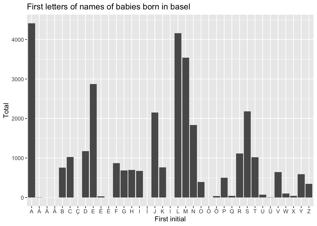
Let’s say we want to know how many Basel babies have names for each letter of the alphabet.
- Use
mutate()to make a new column with the first letter of each name. - Use
group_by()andsummarize()to count the number of babies with each first letter. - Bonus: Make a bar chart of the data, using
ggplot(). You can usegeom_col()to make a bar chart.
Your resulting table should look like this:
| first_letter | total |
|---|---|
| A | 4411 |
| B | 757 |
| C | 1027 |
| D | 1173 |
| E | 2873 |
| F | 868 |
| G | 687 |
| H | 700 |
| I | 675 |
| J | 2154 |
The plot should look like this:
3.12 XLSX
Our last data format for the day is XLSX. This is a proprietary format, and is used by Microsoft Excel. I’d discourage your form using this unless you have to, but sometimes you’ll find it in the wild, and you might have less gifted colleagues who insist on using it.

Let’s download and take a look at some XLSX data, originally from the US Census Bureau:
download.file(
  "https://www2.census.gov/programs-surveys/decennial/2020/data/apportionment/apportionment-2020-table02.xlsx",
  "input_data/state_population.xlsx"
)
Normally, I am a big advocate for looking at the plain text of files before you import them, but XLSX files are a little different. They’re actually a zip file, with a bunch of XML files inside. If you try to open them in a text editor, you’ll just see a bunch of gibberish.
Of course, you can always open them in Excel, but that’s not very reproducible. Instead, we’ll use the readxl package to read the data into R.
Load the library in the usual way:
Now, you can click on your downloaded file in the file editor, and import it just like you did with the CSV file. You can see complete instructions in the last chapter.
The code that we get back should look something like this:
Let’s take a look at the data frame we get back:
## # A tibble: 6 × 3
## AREA `RESIDENT POPULATION (APRIL 1, 2020)` This cell is intentionally …¹
## <chr> <dbl> <lgl>
## 1 Alabama 5024279 NA
## 2 Alaska 733391 NA
## 3 Arizona 7151502 NA
## 4 Arkansas 3011524 NA
## 5 California 39538223 NA
## 6 Colorado 5773714 NA
## # ℹ abbreviated name: ¹`This cell is intentionally blank.`We have three columns:
- AREA
- RESIDENT POPULATION (APRIL 1, 2020)
- This cell is intentionally blank.
First, let’s rename the columns to something a little more sensible:
Next, we can get rid of the blank column. A quick way to do this is to use the select() function
with a minus sign in front of the column name that we don’t want:
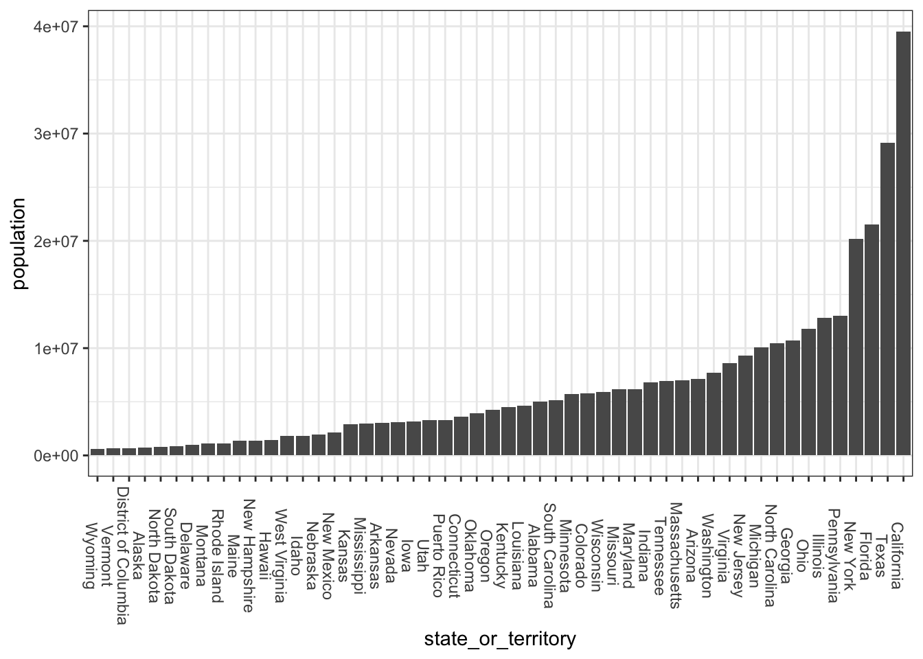
When we look at the data frame, we can see that the last few rows should be removed, but maybe Puerto Rico should be included in our calculations. 8
| state_or_territory | population |
|---|---|
| Wisconsin | 5893718 |
| Wyoming | 576851 |
| TOTAL RESIDENT POPULATION1 | 331449281 |
| Puerto Rico | 3285874 |
| TOTAL RESIDENT POPULATION, INCLUDING PUERTO RICO | 334735155 |
| Footnote: 1 Includes the resident population for the 50 states and the District of Columbia, as ascertained by the Twenty-Fourth | |
| Decennial Census under Title 13, United States Code. | NA |
There are a couple ways we could do this, but for now let’s:
- Make a new data frame with just P.R.
- Remove the last 5 rows of the data frame.
- Combine the two data frames.
- Remove the P.R. dataframe from memory.
First, we use filter() to make a 1-row data frame with just Puerto Rico:
puerto_rico_temp <- state_population |>
  filter(state_or_territory == "Puerto Rico")
puerto_rico_temp
## # A tibble: 1 × 2
## state_or_territory population
## <chr> <dbl>
## 1 Puerto Rico 3285874Second, we can use head() to select the first 51 rows of the data frame:
## # A tibble: 51 × 2
##    state_or_territory   population
##    <chr>                     <dbl>
##  1 Alabama                 5024279
##  2 Alaska                   733391
##  3 Arizona                 7151502
##  4 Arkansas                3011524
##  5 California             39538223
##  6 Colorado                5773714
##  7 Connecticut             3605944
##  8 Delaware                 989948
##  9 District of Columbia     689545
## 10 Florida                21538187
## # ℹ 41 more rows
Third, we row-bind the two data frames together:
## # A tibble: 6 × 2
##   state_or_territory population
##   <chr>                   <dbl>
## 1 Virginia              8631393
## 2 Washington            7705281
## 3 West Virginia         1793716
## 4 Wisconsin             5893718
## 5 Wyoming                576851
## 6 Puerto Rico           3285874
When we look at the tail of the data frame, we can see that Puerto Rico is now included.
Finally, we remove the temporary data frame from memory:
This, if you want, could be plotted like so:
You can type 1e6 instead of 1000000, if you don’t like counting zeros↩︎
Don’t do this in real life, just look up the population↩︎
For now, don’t worry what
simplifyVectordoes.↩︎R is friendly to both Brits and Americans, so it has both the
summarise()andsummarize()functions, which do the exact same thing.↩︎https://en.wikipedia.org/wiki/Political_status_of_Puerto_Rico↩︎