8 RMarkdown
This extra chapter is dedicated to RMarkdown which will be used for producing your final report during the exam.
8.1 RMarkdown
RMarkdown is the best framework for data science (official website: https://rmarkdown.rstudio.com/). It makes it possible to obtain reproducible reports that include text, R code and the corresponding output. See this video for an introduction to RMarkdown: https://vimeo.com/178485416. To use RMarkdown you have to install the rmarkdown and knitr package.
For the C4DS exam you will receive a RMarkdown document, i.e. a file with .Rmd extension (see for example the file C4DS_Exam_FacSimile.Rmd available in the Moodle page). You can open the file (by double clicking) with RStudio.
In the top part of the file, as shown in Figure 8.1, you just have to write your Surname, Name and Student ID. The rest must not be modified. You can compile the RMarkdown file to obtain an html file by using the Knit button, see the yellow circle in Figure 8.1. If the compilation concludes correctly a web page will be opened with your html browser. Moreover, the file C4DS_Exam_FacSimile.html will be created in the same folder where the RMarkdown file is saved. If you want to see the web page directly in the bottom right panel of RStudio (Viewer pane) click on the wheel button (see the purple circle in Figure 8.1) and select Preview in Viewer Pane (then compile again your document with Knit, you will see your document in the Viewer pane).
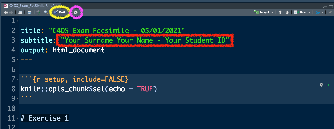
Figure 8.1: Top part of the RMarkdown file
In Figure 8.2 you can view the beginning of Exercise 1 (see the purple rectangle) and the first sub-exercise (1.). This must not be modified. You have instead to write your code and your comments (preceded by #) in the yellow area delimited by the symbols ```{r} and ``` (this area is known as code chunk). To check what your code produces you can:
- run separately each line of code by using Ctrl/Cmd Enter. This is the approach you have used so far, you will find your results in the console and the new objects in your environment (see top right panel).
- Use the arrow located in the right part of the code chunk (see the orange arrow in Figure 8.2 ). This will run all the code lines included in the chunk. You will find your results in the console and the new objects in your environment (see top right panel).
In any case you have to compile your document (using the Knit button) after each sub-exercise. This will make you possible to check the final html file step by step. At the end of your exam you will have to deliver both the .Rmd and .html file (you will upload them to the Moodle page).
Remember that if a code gives you errors or doesn’t work you can always keep it in your .Rmd file by commenting it out.
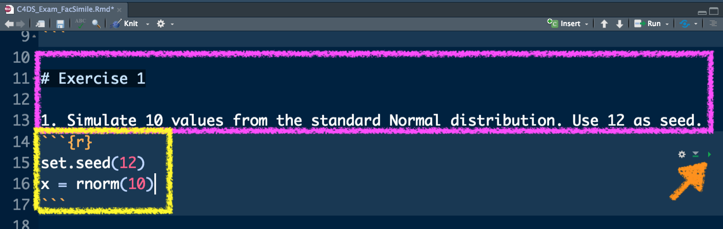
Figure 8.2: Text of an exercise in RMarkdown and code chunk
8.2 Extra exercises
Solve the exercises contained in the RMarkdown file R_Lab_Extra_empty.Rmd. At the end you should obtain an html file with your solutions. For the exercises you can decide to use a standard or tidyverse-based R coding.