5 Lecture 3 - 15/12/2020
In this lecture we will learn how to write new functions in R.
5.1 Create a new data frame
We start by creating a new data frame from scratch. Differently from Lecture 2, we don’t import data available in an external (csv) file, but we put together data simulated from 4 different random variables (RV). In particular, we will simulate 500 values from each of the following RVs:
- standard Normal distribution (
rnorm(n,mean,sd)) - continuous Uniform distribution between 0 and 10 (
runif(n,min,max)) - t distribution with 4 degrees of freedom (
rt(n,df)) - Chi-square distribution with 5 degrees of freedom (
rchisq(n,df))
As discussed in Section XXXX, before running the data simulation code we set the seed. Then, the function data.frame is used to combine the 4 vectors (named x, y, w and z) generated by the 4 functions for random sampling. The data frame will be called df:
set.seed(56)

df = data.frame(x = rnorm(500),
                y = runif(500, 0, 10),
                w = rt(500, 4),
                z = rchisq(500, 5))
From the preview
##            x         y          w        z
## 1 -0.2409516 6.4480150 -1.1082764 2.464180
## 2 -0.5004062 9.9065245 -2.3763105 6.582193
## 3 -0.3952414 3.4989756 -1.4033463 5.045619
## 4 -0.7952692 0.9429413  0.7804105 4.606289
## 5  0.5399611 5.1325526  0.8343994 4.209044
## 6  1.4889313 5.1903847  2.1541173 2.229942
we observe that the data frame contains 4 columns.
As shown in Lecture 2, it is possible to compute the mean for all the columns of the data frame, as follows:
##           x           y           w           z
## -0.05370359  4.93485392  0.01570831  4.96757021
5.2 Skewness index
The formula for the skewness index of a generic variable \(x\) is the following \[ sk = \frac{\frac{\sum_{i=1}^n (x_i-\bar x)^3}{n}}{s^3} \] where \(s\) is the sample standard deviation and \(n\) the sample size.
Note that there is no buil-in function for computing the skewness in R. So, we implement the above given equation, separately for each column in df, as follows:
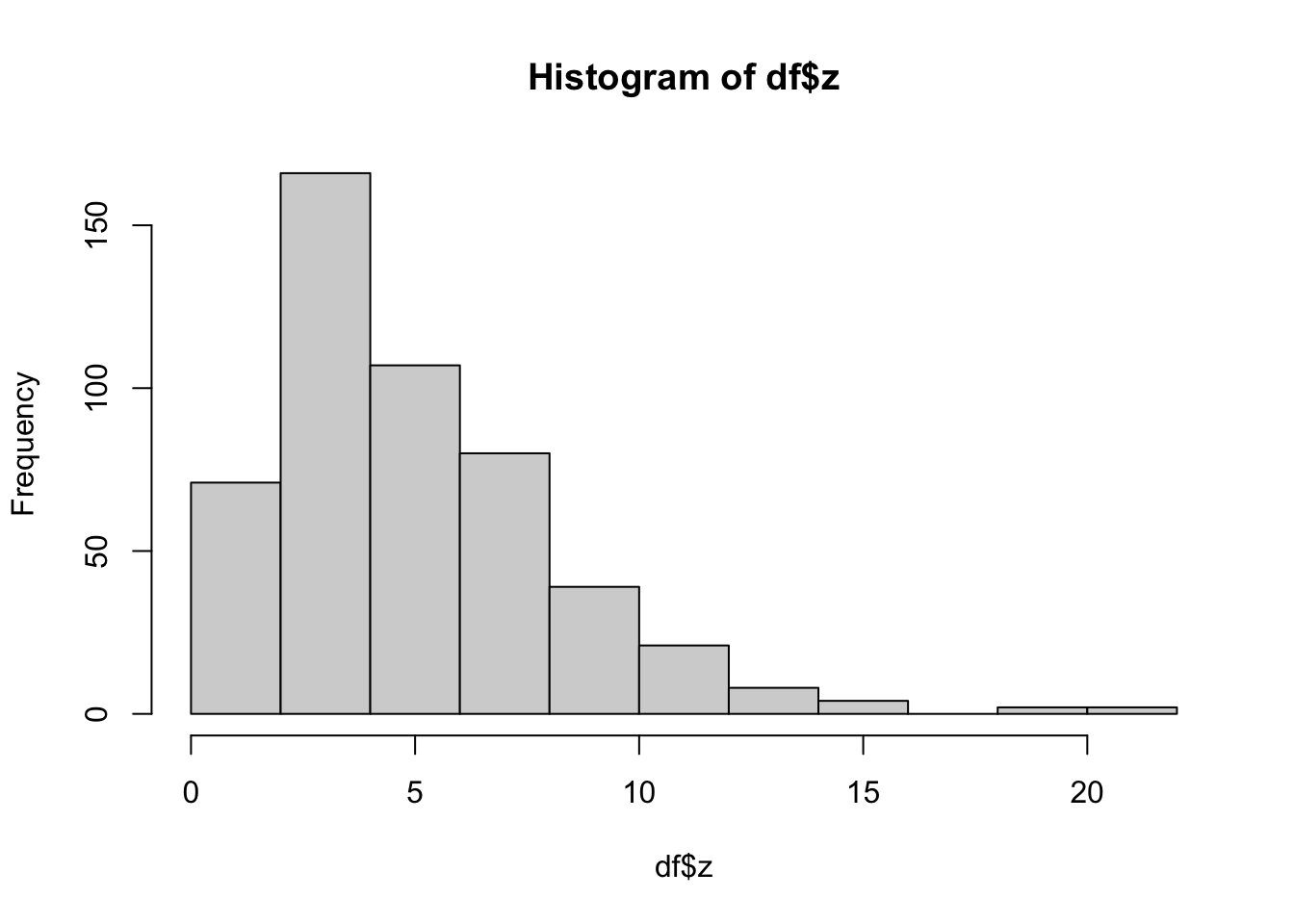
## [1] -0.1391724## [1] 0.00426134## [1] -0.2061976## [1] 1.367381The variable z is characterized by positive skewness, which is also visible from the following histogram:
5.3 Write a new function in R
The Do not repeat yourself (DRY) principle suggests avoiding repetitions in the code, as copy-and-paste the same code to compute the same quantity(ies) for different data, as we did previously for the skewness index. The more repetition you have in your code, the more places you need to remember to update when things change, and the more likely you will include errors in your code.
Automate common tasks through functions is a powerful alternative to copy-and-paste. When input changes, with functions you only need to update the code in one place instead of many (this eliminates the chance of incidental mistakes).
To define a new function we use the following structure: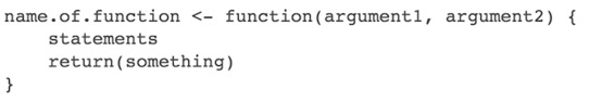
Figure 5.1: How to define a new function with 2 inputs in R
For the computation of the skewness index we define a new function named myskew which take in input the vector named vec and then apply the skewness formula:
After running the code, you will see a new object of type function in the top right panel. It is now possible to apply the function to a single column of df:
## [1] -0.1391724You can even use myskew inside apply:
##           x           y           w           z
## -0.13917239  0.00426134 -0.20619759  1.36738140
Note that by default the function returns the value of the last evaluated expression (the value of the skewness index in this case). Let’s assume that we want to define a new function which returns the values of the skewness and kurtosis indexes. In this case the output is a vector of two values (s and k representing the skewness and kurtosis index, respectively) and it can be returned by using the return function:
myskewkur = function(vec){
  s = mean((vec - mean(vec))^3) / sd(vec)^3
  k = mean((vec - mean(vec))^4) / sd(vec)^4
  return(c(s,k))
}
Let’s now apply the function myskewkur to a single column of df and to all its column by using apply:
## [1] -0.1391724 2.7668950## x y w z
## [1,] -0.1391724 0.00426134 -0.2061976 1.367381
## [2,] 2.7668950 1.82261893 6.0524876 5.895259We can observe that the output is not labeled. It is possible to obtain a labeled output by changing the returned vector and including labels:
myskewkur = function(vec){
  s = mean((vec - mean(vec))^3) / sd(vec)^3
  k = mean((vec - mean(vec))^4) / sd(vec)^4
  return(c("skewness"=s,"kurtosis"=k))
}
The output now is completely specified:
##   skewness   kurtosis
## -0.1391724 2.7668950## x y w z
## skewness -0.1391724 0.00426134 -0.2061976 1.367381
## kurtosis 2.7668950 1.82261893 6.0524876 5.8952595.3.1 Conditional statement
Let’s say that we want now our function to print a message according to the value of skewness and kurtosis. In particular, if the skewness is positive the function prints “Data with positive asymmetry”; otherwise the function prints “Data with null or negative asymmetry”. For the kurtosis the function will print “Data with heavier tails” or “Data with lighter or Normal tails” according to the value being bigger or lower than 3 (the reference kurtosis value for the Normal distribution). For obtaining this conditional output (conditional on the value of the skewness/kurtosis), we will use the function ifelse as described in Lecture 2:
myskewkur2 = function(vec){
  s = mean((vec - mean(vec))^3) / sd(vec)^3
  k = mean((vec - mean(vec))^4) / sd(vec)^4

  ifelse(s>0,
         print("Data with positive asymmetry"),
         print("Data with null or negative asymmetry"))

  ifelse(k>3,
         print("Data with heavier tails"),
         print("Data with lighter or Normal tails"))

  return(c("skewness"=s,"kurtosis"=k))
}
We can use now the function:
## [1] "Data with null or negative asymmetry"
## [1] "Data with lighter or Normal tails"
## skewness kurtosis
## -0.1391724 2.7668950Sometimes what you have to execute, conditionally on a given conditions, it is more complex than just a simple print command. In this case you will need another kind of conditional statement, as the following one:
if (condition){
  expr1
  #code executed when condition is TRUE
} else {
  expr2
  #code executed when condition is FALSE
}
Using this structure the same function could be rewritten as follows:
myskewkur3 = function(vec){
  s = mean((vec - mean(vec))^3) / sd(vec)^3
  k = mean((vec - mean(vec))^4) / sd(vec)^4

  if(s>0){
    print("Data with positive asymmetry")
  } else {
    print("Data with null or negative asymmetry")
  }

  if(k>3){
    print("Data with heavier tails")
  } else {
    print("Data with lighter tails")
  }

  return(c("skewness"=s,"kurtosis"=k))
}
The output will be the same:
## [1] "Data with null or negative asymmetry"
## [1] "Data with lighter tails"
## skewness kurtosis
## -0.1391724 2.7668950It is also possible to test more conditions:
5.4 Again about factors
We now add a new column to the dataframe df given by a vector of 500 categories randomly sampled from “Low”, “Medium” and “High”. We will make use of the function sample (see ?sample); it takes a sample of the specified size (500) from the elements of the vector with the 3 categories with replacement (so each category can be sampled more than once). As described in Lecture 2 we immediately transform this character vector into a factor:
Let’s check the new column in df:
##            x         y          w        z   size
## 1 -0.2409516 6.4480150 -1.1082764 2.464180   High
## 2 -0.5004062 9.9065245 -2.3763105 6.582193 Medium
## 3 -0.3952414 3.4989756 -1.4033463 5.045619   High
## 4 -0.7952692 0.9429413  0.7804105 4.606289 Medium
## 5  0.5399611 5.1325526  0.8343994 4.209044 Medium
## 6 1.4889313 5.1903847 2.1541173 2.229942 Low## 'data.frame': 500 obs. of 5 variables:
## $ x : num -0.241 -0.5 -0.395 -0.795 0.54 ...
## $ y : num 6.448 9.907 3.499 0.943 5.133 ...
## $ w : num -1.108 -2.376 -1.403 0.78 0.834 ...
## $ z : num 2.46 6.58 5.05 4.61 4.21 ...
## $ size: Factor w/ 3 levels "High","Low","Medium": 1 3 1 3 3 2 2 1 1 3 ...We know that it is possible to apply the function summary to a factor in order to obtain the frequency distribution. It can also be obtained by using table:
##   High    Low Medium
## 155 187 158##
## High Low Medium
## 155 187 158If you are interested in proportions/percentages, rather than absolute frequencies, we can use the function prop.table:
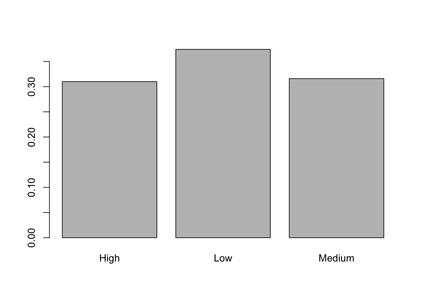
##
##   High    Low Medium
##   31.0   37.4   31.6
It is also possible to represent graphically the distribution of the categorical variable size by using barplot:

5.5 Exercises Lecture 3
5.5.1 Exercise 1
Define a function named
mypowerto print a number raise to another. The two numbers are the arguments of the function and the exponent number is set by default equal to one.Compute using
mypowerthe following quantities: \(2^3\), \((\exp(4))^\sqrt{5}\), \(\log(45)\).Is it possibile to provide a vector of exponents as input to the
mypowerfunction (while the base doesn’t change)? If yes, provide and example.
5.5.2 Exercise 2
- Define a function named
myfwhich takes a single argument \(x\) and returns the value of the function \(f(x)\) which is defined as follows:
- \(f(x)=x^2+2x+3\) if \(x<0\);
- \(f(x)=x+3\) if \(0\leq x <2\);
- \(f(x)=x^2+4x-7\) if \(x\geq 2\).
- Evaluate the function in the following values of \(x\): -4.5, 5.90, 122.
5.5.3 Exercise 3
Define a function which computes, given a sample of \(n\) data, the confidence interval with confidence level \(1-\alpha\) for the unknown mean of the population where the sample is drawn from. For \(1-\alpha\) use 0.95 as default value. Remember that the formula for the confidence interval is given by the following formula: \[\left(\bar x -z_{\alpha/2}\frac{s}{\sqrt n};\bar x +z_{\alpha/2}\frac{s}{\sqrt n}\right)\] where \(\bar x\) is the sample mean (
mean), \(s\) the sample standard deviation (sd), \(n\) the sample size and \(z_{\alpha/2}\) the quantile of the standard Normal distribution which has an area equal to \(1-\alpha/2\) on the left side (use the functionqnormto compute it; see?qnorm).Apply the function to a vector of 600 numbers simulated from a Normal distribution with mean equal to 5 and variance equal to 1. For simulating the data use 444 as seed value.
5.5.4 Exercise 4
Create a function
wt_meanwhich compute the weighted mean given by this formula \[\bar x = \frac{\sum_{i=1}^n x_iw_i}{\sum_{i=1}^n w_i}\] where \(x_i\) is the generic value of the variable and \(w_i\) the corresponding weigth (\(i=1,\ldots,n\)). This function will have two vectors as input (one for the data and one for the weights) and you have to check they they have the same length, otherwise the function will have to stop and exit with an error message (for this you can usestop, see?stop).Test the function with the following data (exam grades) and weights (exam credits):
Test the function with the following data (exam grades) and weights (exam credits):
5.5.5 Exercise 5
Implement a
ratiofunction which takes a single number as input. If the number is divisible by three, it returns “Divisible by 3”. If it’s divisible by five it returns “Divisible by 5”. If it’s divisible by three and five, it returns “Divisible by 3 and 5”. Otherwise, it returns the number. Use the modulo operator%%to check divisibility. The expressionx %% yreturns 0 ifydividesx. See the following example:Run the
ratiofunction with the following numbers: 33, 50, 150, 46570, 9877.Try to understand what the code
y=round(runif(1,0,1000),0)does. Then run (many times) theratiofunction with the valuey.
5.5.6 Exercise 6
- How could you use
cutfunction to simplify this set of nested if-else statements? See?cut. Suggestion: use-InfandInffor the lowest and highest value.
temp = 22.5

if (temp <= 0) {
  "freezing"
  } else if (temp <= 10) {
  "cold"
  } else if (temp <= 20) {
  "cool"
  } else if (temp <= 30) {
  "warm"
  } else {
  "hot"
}
## [1] "warm"- Run the code with
cutwith a vector of temperature, e.g.runif(15, -30,60). Provide the absolute frequencies for the qualitative variable with 5 categories.