7 Lecture 5 - 22/12/2020

In this lecture we will learn how to use the ggplot2 library to produce very nice plots.

7.1 The `ggplot2` library

The ggplot2 is part of the tidyverse collection of packages. The grammar of graphics plot (ggplot) is an alternative to standard R functions for plotting; see here for the ggplot2 website. In Figure ?? we have some examples of plot (simple scatterplot, scatterplot with legend and boxplots) produced using standard R code and the ggplot2 library.

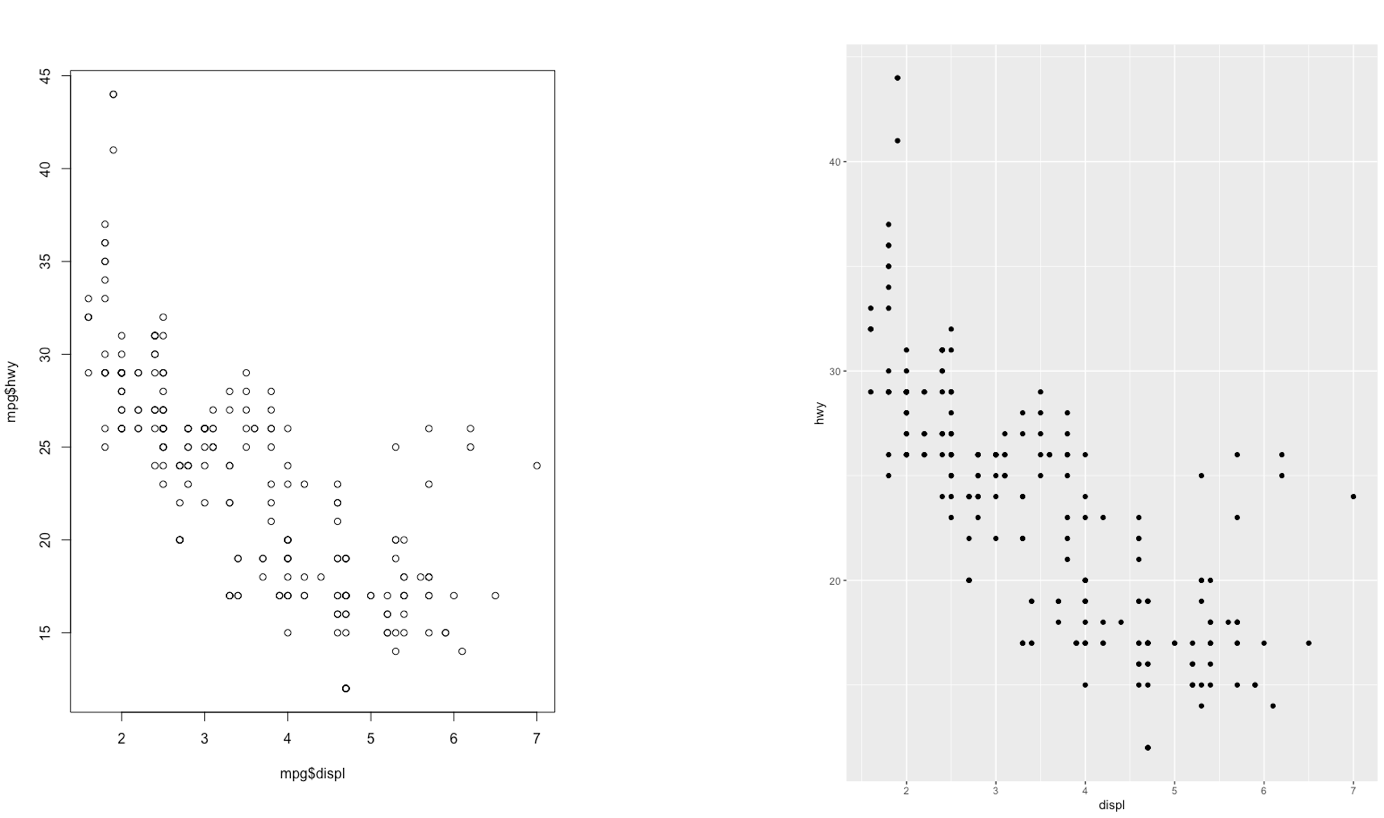
Figure 7.1: Comparison between standard and ggplot2 plots

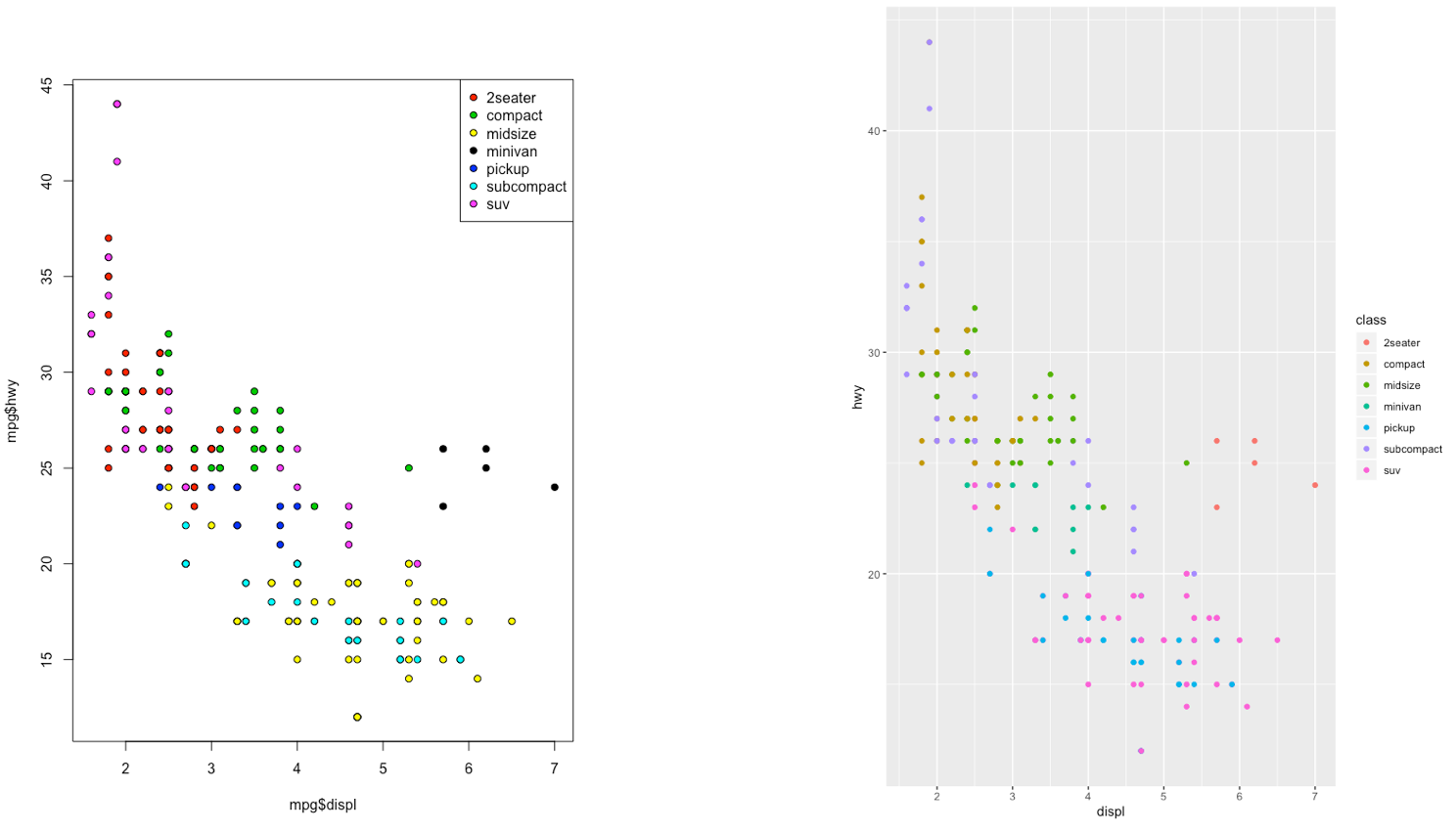
Figure 7.2: Comparison between standard and ggplot2 plots

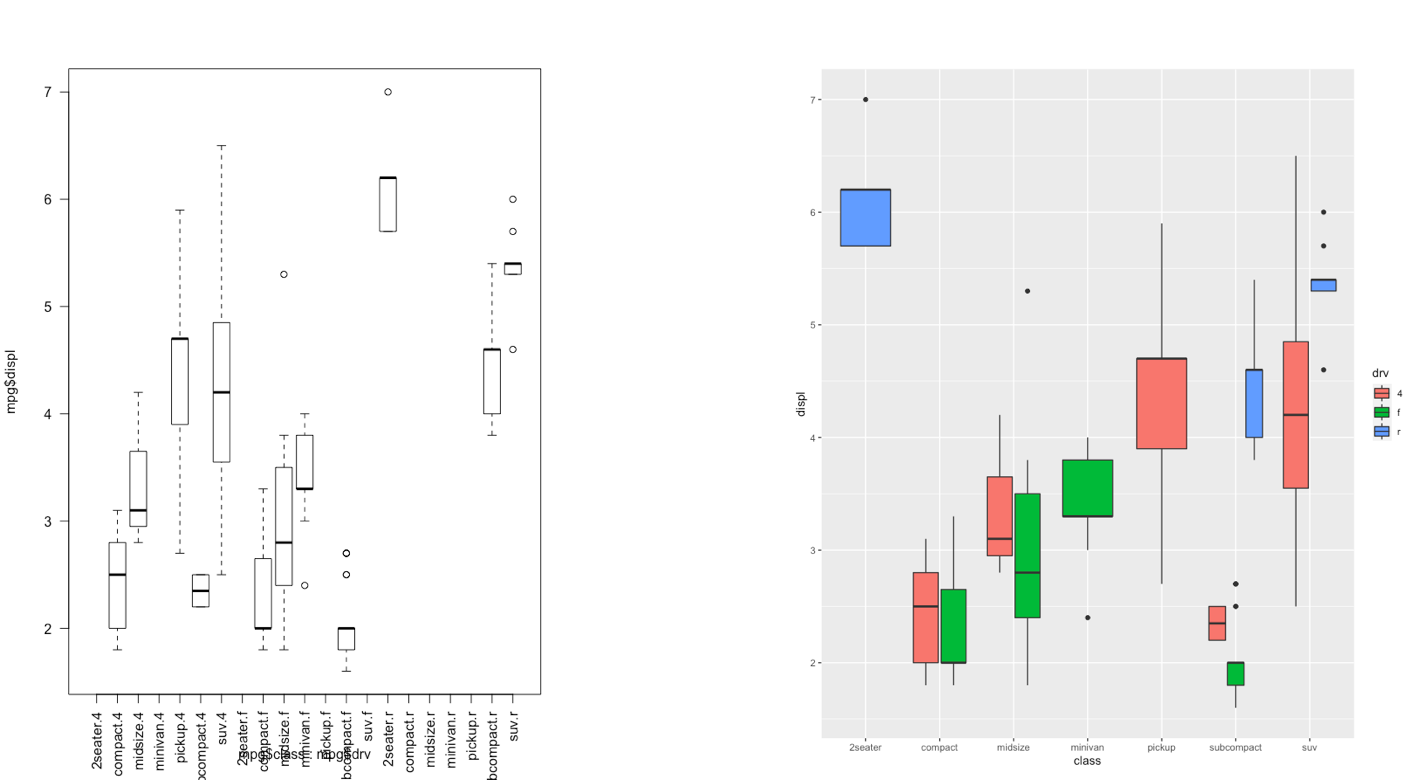
Figure 7.3: Comparison between standard and ggplot2 plots

With ggplot2 a plot is defined by several layers, as shown in Figure 7.4. The first layer specifies the coordinate system, then we can have several geometries each with aesthetics specification.

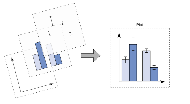
Figure 7.4: The layer structure of the ggplot2 plot

7.2 Data subsetting and the `ggplot` function

Instead of working with the entire diamonds data set, as done in Lecture 4, we will create a smaller data set by sampling randomly 1% of the diamonds by means of the function sample_frac. As this is a random procedure we set, as usual, the seed in order to have a reproducible outcome. The new (smaller) data set will be called mydiamonds:

library(tidyverse)
set.seed(4)
mydiamonds = sample_frac(diamonds, 0.01)
glimpse(mydiamonds)

## Rows: 539
## Columns: 10
## $ carat   <dbl> 0.72, 1.52, 0.32, 1.10, 1.34, 0.31, 0.26, 0.70, 0.36, 0.37, 1.…
## $ cut     <ord> Ideal, Good, Premium, Premium, Ideal, Very Good, Ideal, Premiu…
## $ color   <ord> E, J, G, J, H, G, I, G, E, D, I, H, E, D, G, I, G, G, E, H, D,…
## $ clarity <ord> VS2, VS2, SI1, VS2, SI1, VVS1, VS2, SI1, VS1, SI1, VS1, VS2, V…
## $ depth   <dbl> 62.8, 63.3, 61.0, 61.2, 62.4, 63.0, 62.0, 61.8, 60.9, 62.7, 60…
## $ table   <dbl> 57, 56, 61, 57, 54, 56, 56, 59, 57, 58, 60, 61, 59, 56, 54, 58…
## $ price   <int> 2835, 7370, 612, 3696, 7659, 710, 385, 2184, 782, 874, 6279, 1…
## $ x       <dbl> 5.71, 7.27, 4.41, 6.66, 7.05, 4.26, 4.13, 5.68, 4.60, 4.58, 6.…
## $ y       <dbl> 5.73, 7.33, 4.38, 6.61, 7.08, 4.28, 4.09, 5.59, 4.63, 4.55, 6.…
## $ z       <dbl> 3.59, 4.62, 2.68, 4.06, 4.41, 2.69, 2.55, 3.48, 2.81, 2.86, 4.…

The most important function of the ggplot2 library is the ggplot function. All ggplot plots begin with a call to ggplot supplying the data:

ggplot(data = …) +
  geom_function(mapping = aes(…))

where geom_function is a generic function for a geometry layer; see here for the list of all the available geometries.

For starting a new empty plot we can proceed by using one of the following codes:

ggplot(data=mydiamonds)

ggplot(mydiamonds) #the argument name can be omitted

mydiamonds %>% 
  ggplot() #using the pipe

To add components and layers to the empty plot we will use the + symbol.

7.3 Scatterplot

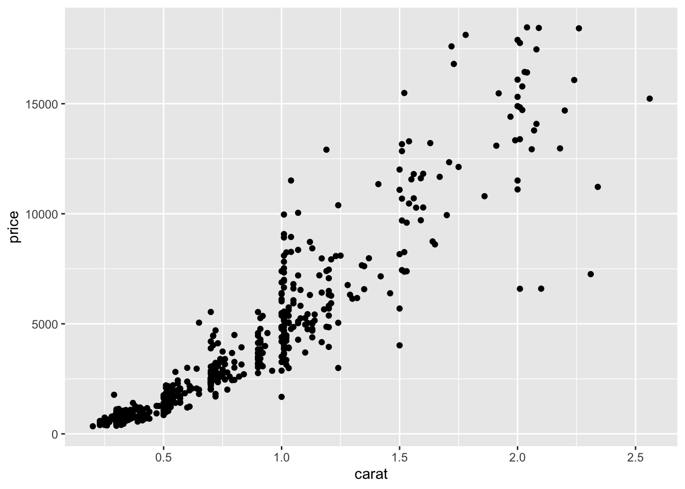
We begin with a scatterplot displaying price on the y-axis and carat on the x-axis; the necessary geometry is implemented with geom_point:

mydiamonds %>% 
  ggplot() +
  geom_point(mapping = aes(x=carat,y=price))

The argument mapping specifies the set of aesthetic mappings, created by aes, which describe the visual characteristics that represent the data, e.g. position, size, color, shape, transparency, fill, etc. From the scatterplot we observe that a positive non linear relationship exists between carat and price.

It is also possible to specify a different color for each point according to the corresponding category of cut:

mydiamonds %>% 
  ggplot() +
  geom_point(mapping = aes(x=carat,y=price,color=cut))

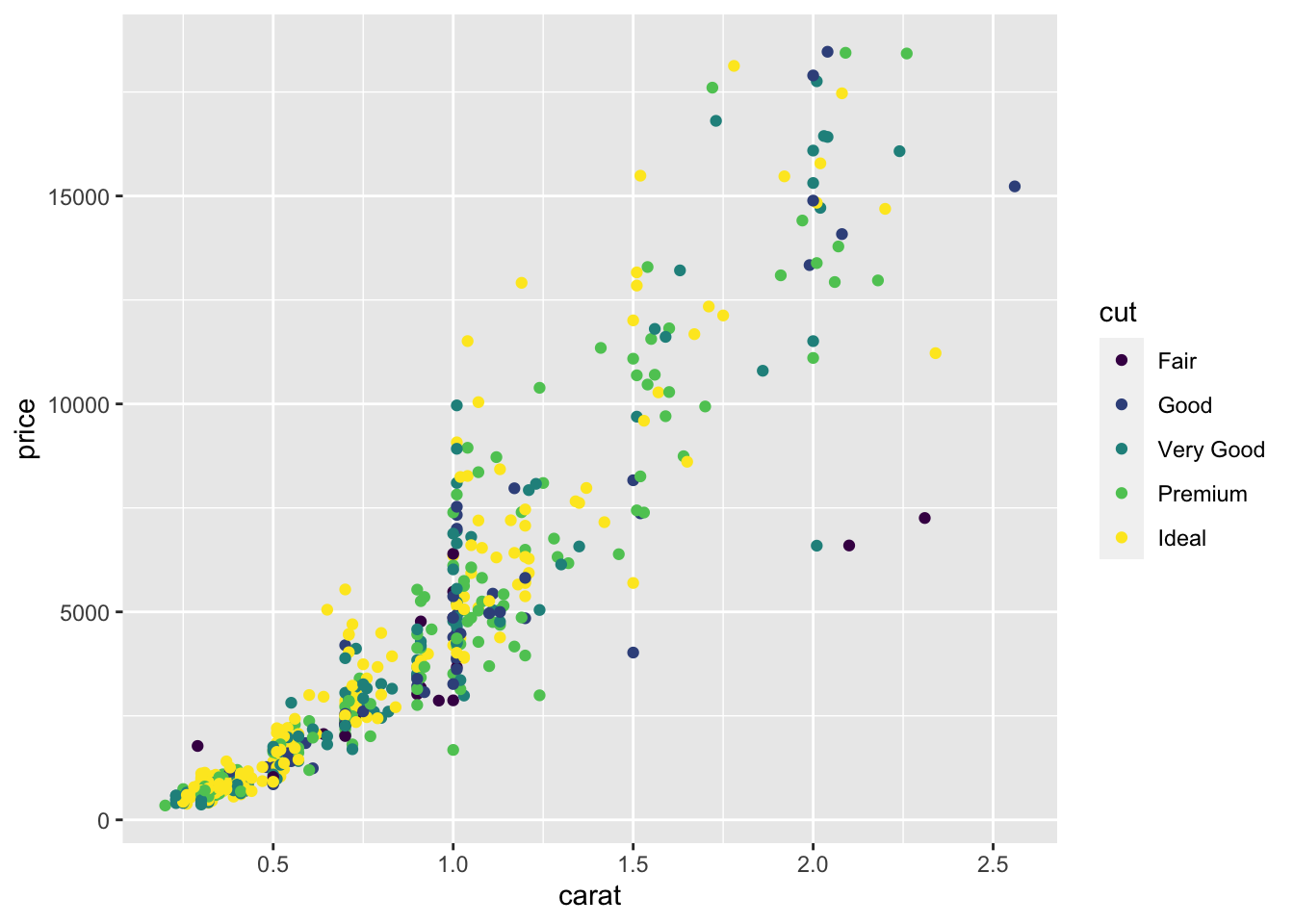Note that automatically a legend is added that explains which level corresponds to each color. From the plot we do not observe a clear clustering of the diamonds according to their quality.

If instead we are interested in changing the point color making all the points blue we have to include the color option outside the aes specification:

mydiamonds %>% 
  ggplot() +
  geom_point(mapping = aes(x=carat,y=price),color="blue")

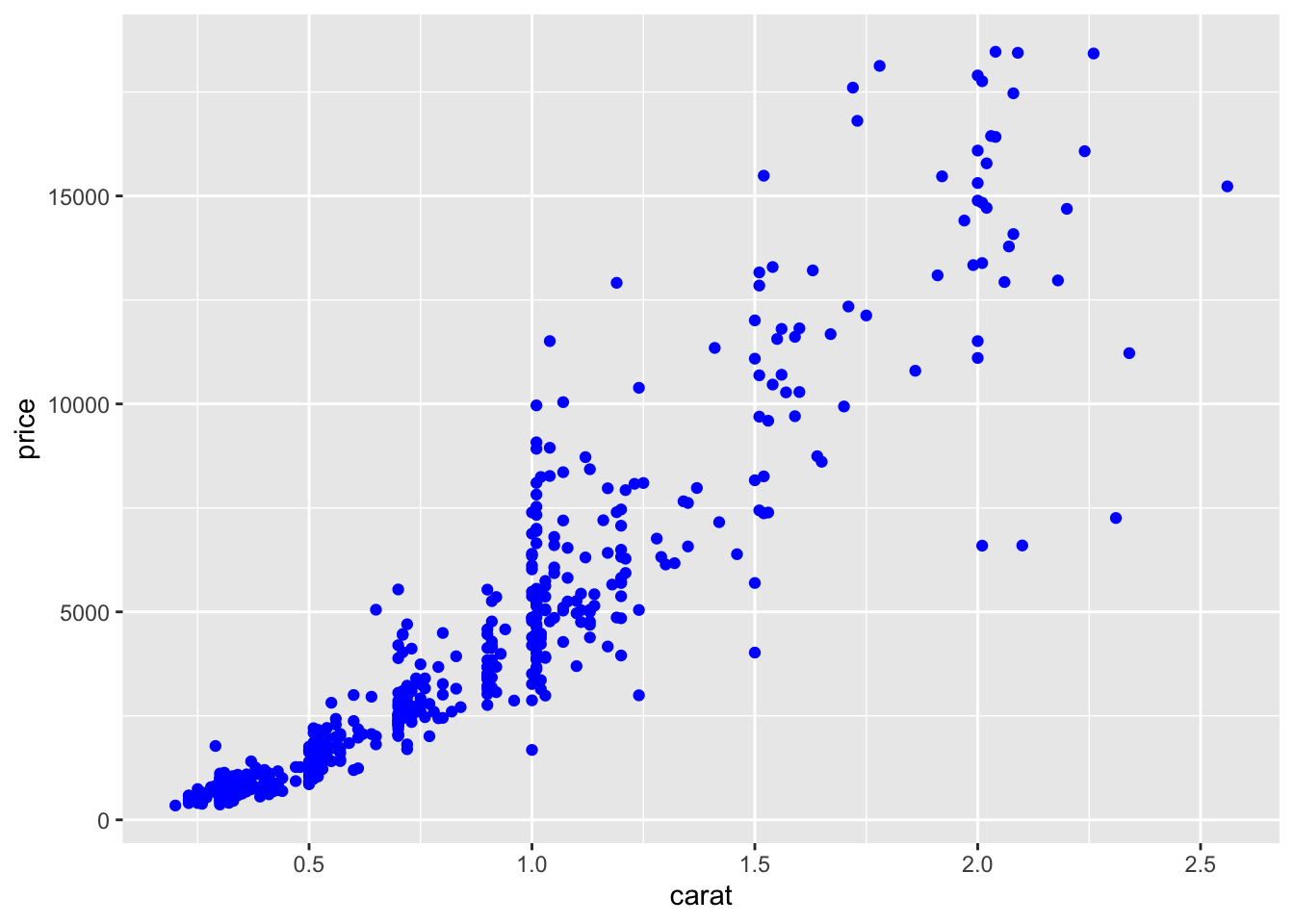Thus, if an aesthetic like the color is linked to data (e.g. cut) it is put into aes(), otherwise it is put outside.

There is also the possibility to set the color according to a condition, e.g. cut == "Premium":

mydiamonds %>% 
  ggplot() +
  geom_point(aes(x=carat, y=price,
                 color = (cut=="Premium")))

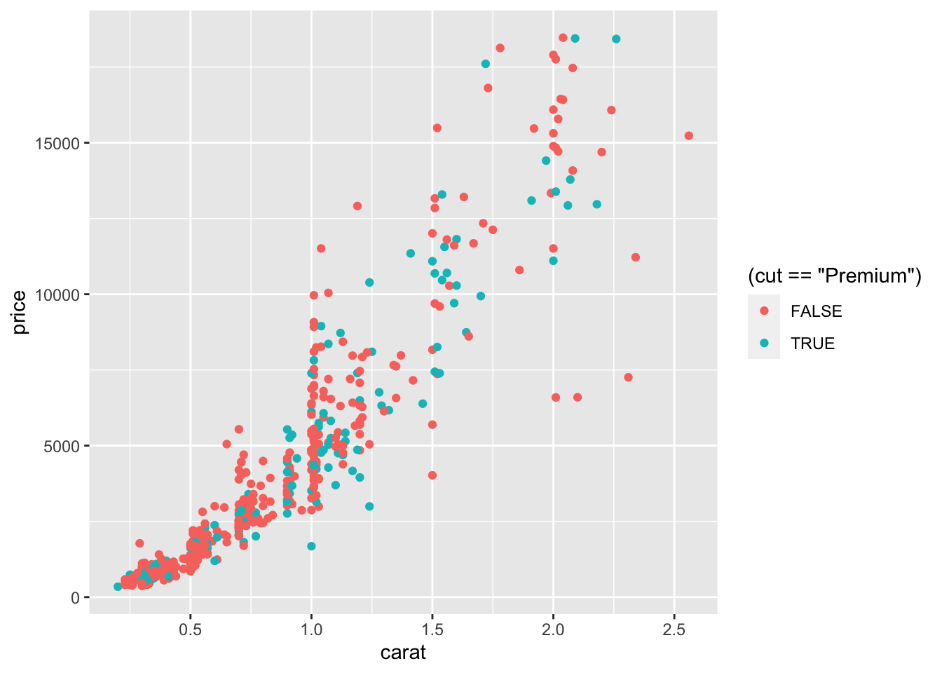In this case the red color is used when the condition is false, and the green color when it is true.

It is also possible to set a different shape - instead of points - according to the categories of cut:

mydiamonds %>% 
  ggplot() +
  geom_point(mapping = aes(x=carat,y=price,shape=cut),
             color="blue")

## Warning: Using shapes for an ordinal variable is not advised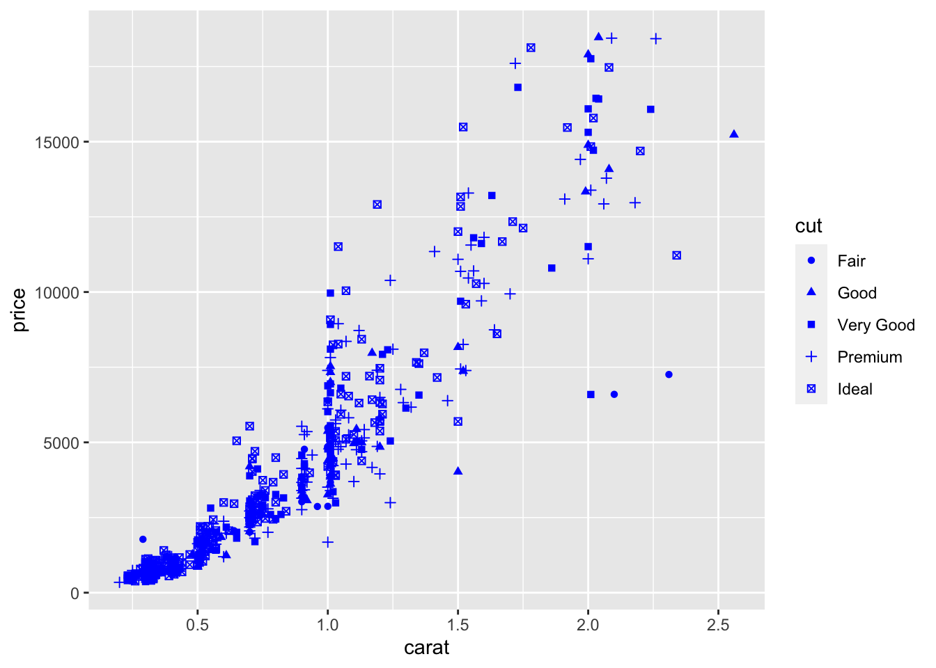

Finally, an alternative for considering the distribution of carat and price conditionally on cut is to produce 5 separate scatterplots according to the 5 categories of cut. In this case we use the facet which defines how data are split among panels. The default facet puts all the data in a single panel, while facet_wrap and facet_grid() allow you to specify different types of small multiple plot.

mydiamonds %>% 
  ggplot() +
  geom_point(mapping = aes(x=carat,y=price), color="blue") +
  geom_smooth(aes(x=carat,y=price)) +
  facet_wrap(~cut)

## `geom_smooth()` using method = 'loess' and formula 'y ~ x'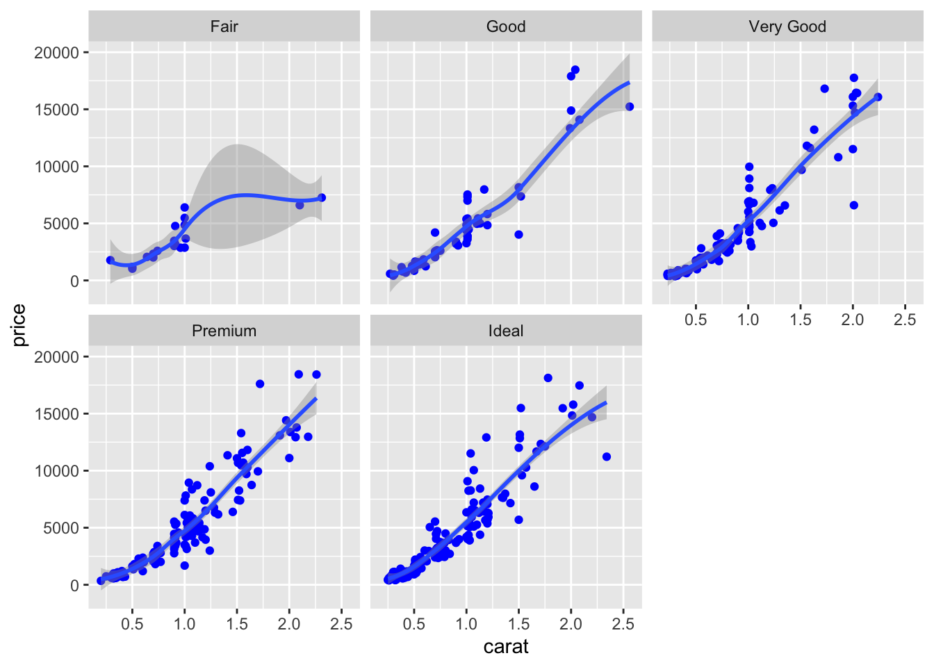

Note that in all the facets reported in the previous plot a new geometry has been included by means of geom_smooth, which adds in the plot a smooth line that can be ease the interpretation of the pattern in the plots.

7.4 Boxplot

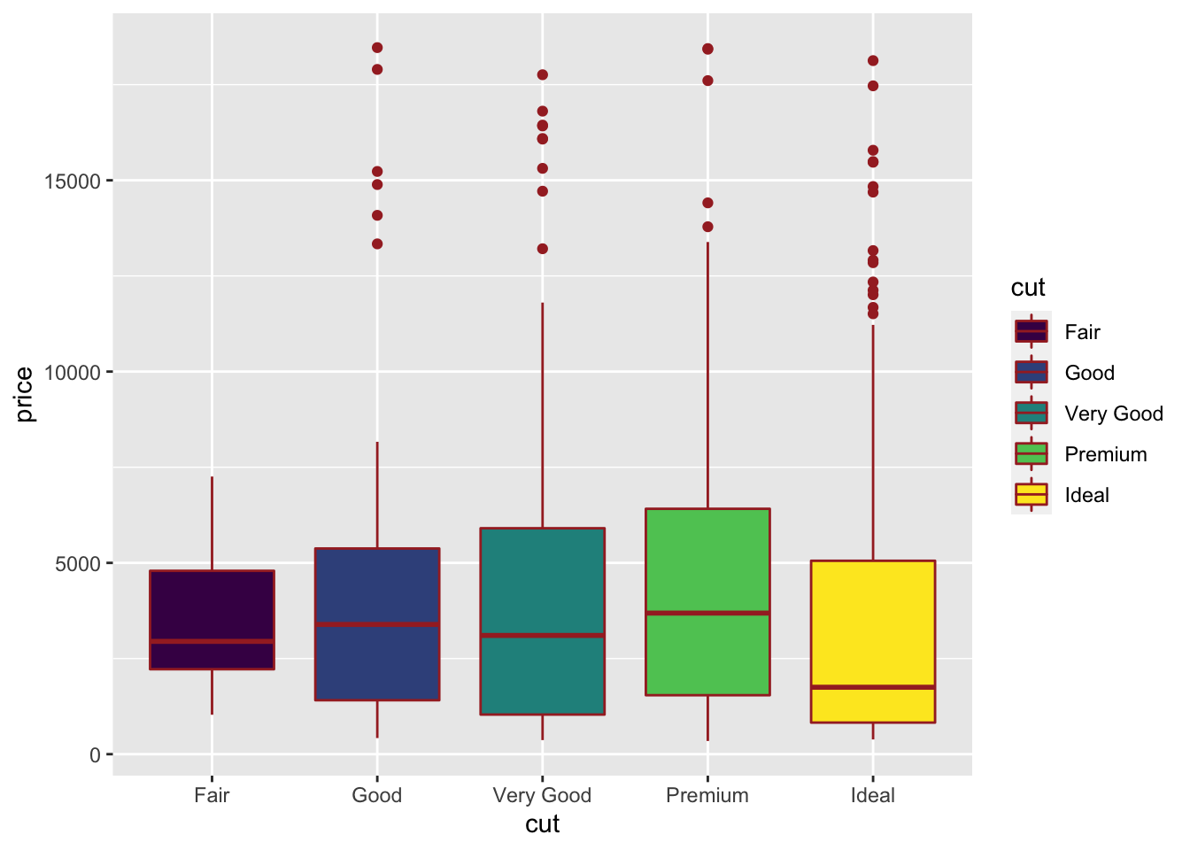
The boxplot can be used to study the distribution of a quantitative variable (e.g. price) conditioning on the categories of a factor (e.g. cut). It can be obtained by using the geom_boxplot geometry, where x is given by the qualitative variable:

mydiamonds %>% 
  ggplot() +
  geom_boxplot(aes(x=cut,y=price))

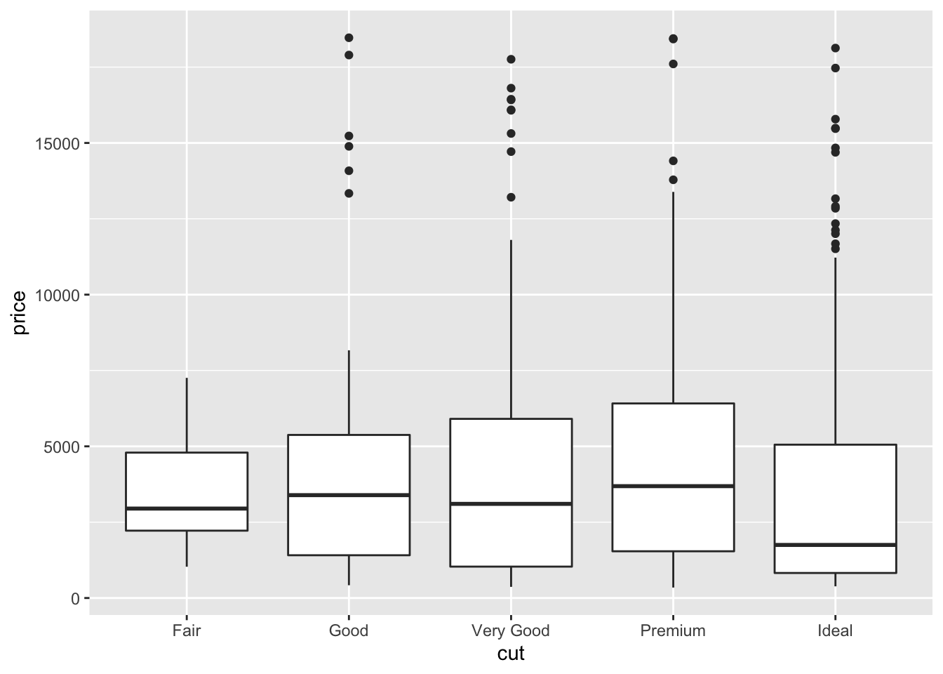The quality category with highest (lowest) median price is Premium (Ideal). Fair quality diamonds are characterized by less variability in terms of price and are not characterized by extreme price values as happened for the other categories.

It is also possible to choose a different fill color and contour color for all the boxes by using fill and color:

mydiamonds %>% 
  ggplot() +
  geom_boxplot(aes(x=cut,y=price),
               fill="red",color="brown")

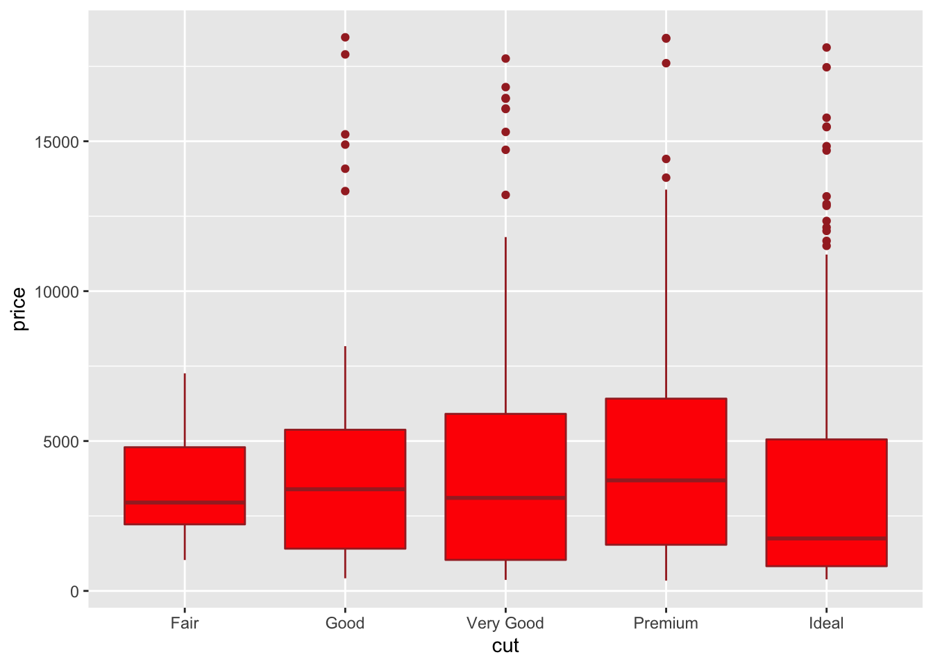
In the previous plot all the boxes are characterized by the same fill and contour color. If we instead interested in using different fill colors according to cut we have to specify the aesthetics with aes:

mydiamonds %>% 
  ggplot() +
  geom_boxplot(aes(x=cut,y=price,fill=cut),
               col="brown")

7.5 Histogram and density plot

When the aim is the analysis of the distribution of a continuos variable like price an histogram can be used. This is implemented by using the geom_histogram geometry:

mydiamonds %>% 
  ggplot() +
  geom_histogram(aes(x=price),
                 fill="lightblue",color="black")

## `stat_bin()` using `bins = 30`. Pick better value with `binwidth`.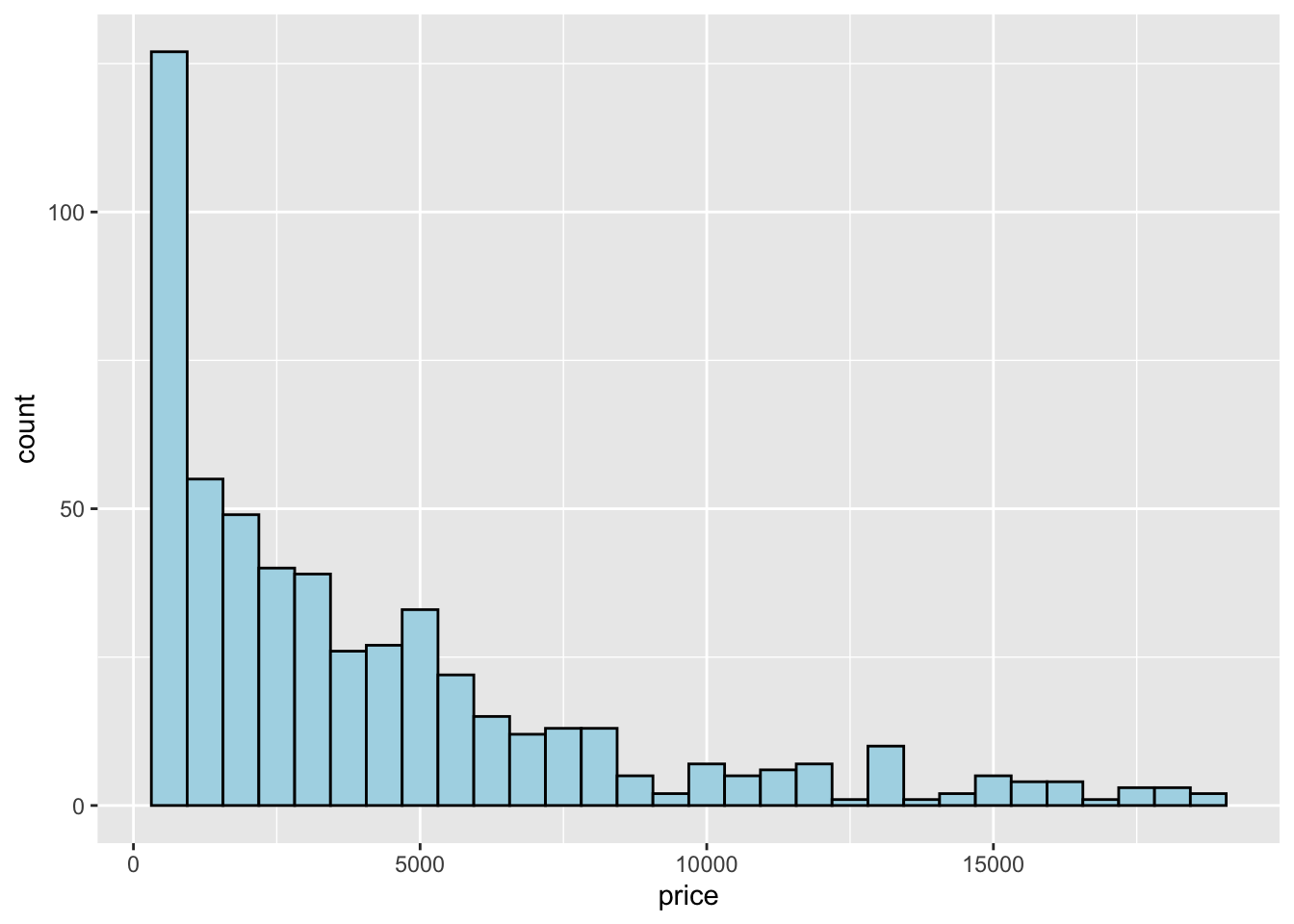

Note that in this case we need to specify only the x variable, while the y is computed automatically by ggplot and corresponds to the count variable (i.e. how many observations for each class of price values). This is given by the fact that every geometry has a default stat specification. For the histogram the default computation is stat_bin which uses 30 bins and computes the following variables: - count, the number of observations in each bin; - density, the density of observations in each bin (percentage of total / bar width); - x, the centre of the bin.

The histogram is a fairly crude estimator of the variable distribution. As an alternative it is possible to use the (non parametric) Kernel Density Estimation (see here) implemented in ggplot by geom_density (only x has to be specified):

mydiamonds %>% 
  ggplot() +
  geom_density(aes(x=price))

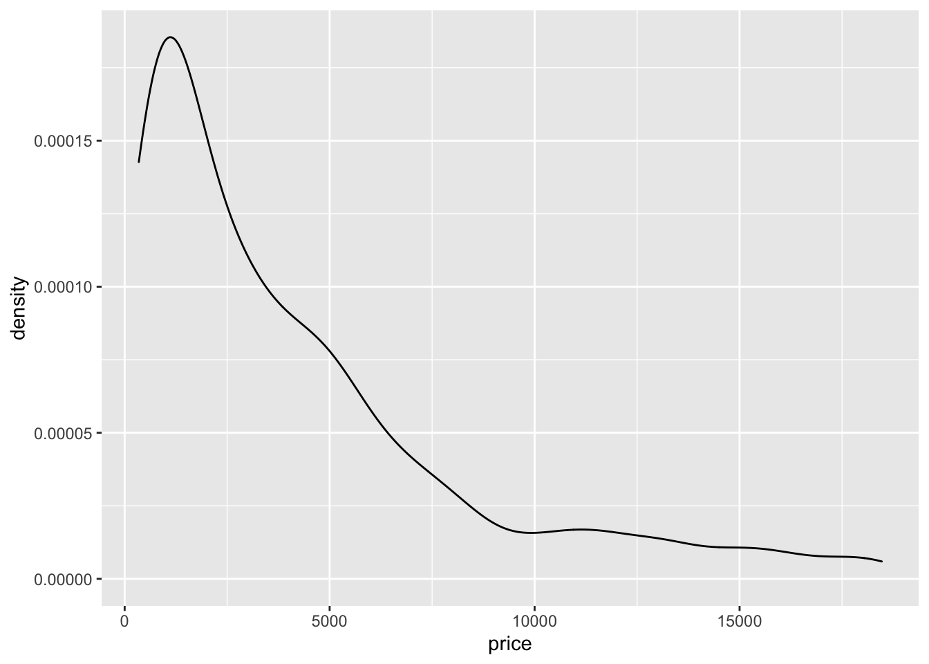Note that the y-axis range is completely different with respect to the one of the histogram.

To combine together in a single plot the histogram and the density function, it is first of all necessary to produce an histogram which uses on the y-axis density instead of counts. The old approach to obtain density also in the y-axis of the histogram uses y=..density... A more modern approach adopts the function after_stat which refers to the generated variable density:

mydiamonds %>% 
  ggplot() +
  geom_histogram(aes(x=price,y=after_stat(density)),
                 fill="lightblue",color="black") +
  geom_density(aes(x=price))

## `stat_bin()` using `bins = 30`. Pick better value with `binwidth`.

Note that the aes settings can be specified separately for each layer or globally in the ggplot function. See here below for a different specification (global now) of the previous plot:

mydiamonds %>% 
  ggplot(aes(x=price)) + # your global specifications
  geom_histogram(aes(y=after_stat(density)),
                 fill="lightblue",color="black") +
  geom_density()

## `stat_bin()` using `bins = 30`. Pick better value with `binwidth`.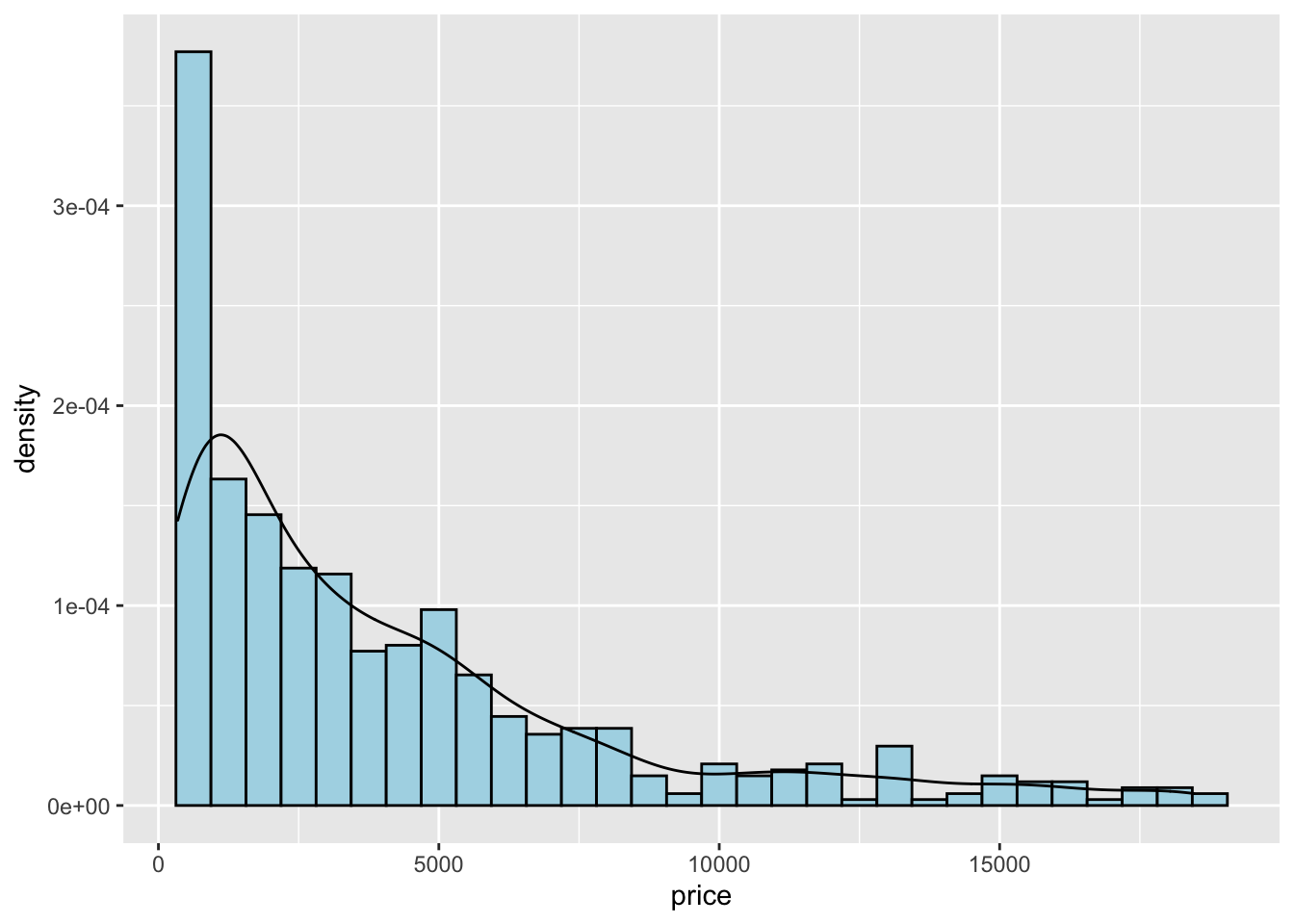

7.6 Barplot

The barplot can be used to represent the distribution of a categorical variable, such as for example cut. It can be obtained by using the geom_bar geometry:

mydiamonds %>% 
  ggplot() +
  geom_bar(aes(x=cut))

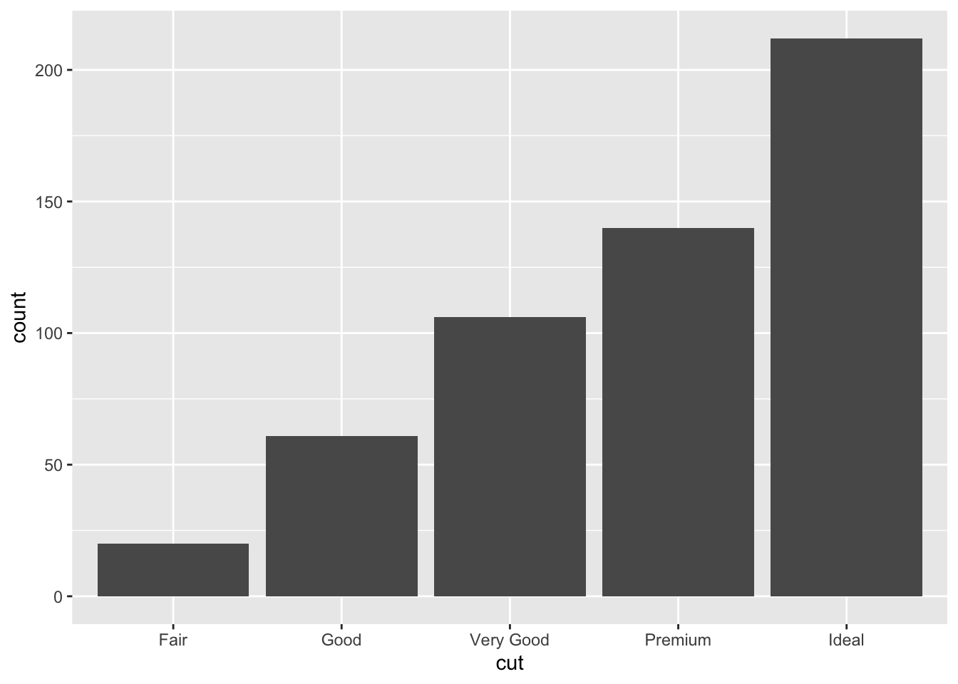Similarly to the histogram, the y-axis is computed automatically and is given by counts (for geom_bar we have that stat="count"). If we are interested in percentages instead of absolute counts we can use the after_stat function and compute a transformation of count:

mydiamonds %>% 
  ggplot() +
  geom_bar(aes(x=cut,
               y=after_stat(count/nrow(mydiamonds)*100)))+
  ylab("my y-axis label") +
  xlab("my x-axis label")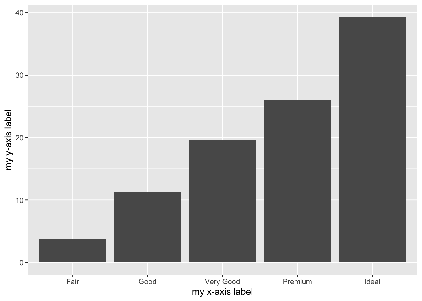

The functions xlab and ylab can be used to specify a different label for the two axes.

It is also possible to take into account in the barplot another qualitative variable such as for example clarity that will be used to set the bar fill aesthetic:

mydiamonds %>% 
  ggplot() +
  geom_bar(aes(x=cut, fill=clarity))

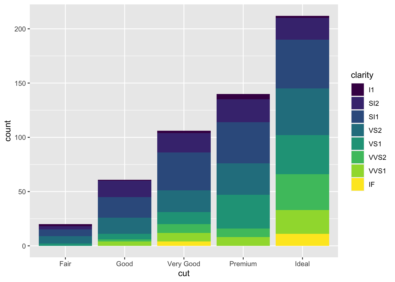Note that the bars are automatically stacked and each colored rectangle represents a combination of cut and clarity. The stacking is performed automatically by the position adjustment given by the position argument (by default it is set to position = "stack"). Other possibilities are "dodge" and "fill":

mydiamonds %>% 
  ggplot() +
  geom_bar(aes(x=cut, fill=clarity), 
           position = "dodge")

mydiamonds %>% 
  ggplot() +
  geom_bar(aes(x=cut, fill=clarity), 
           position = "fill")

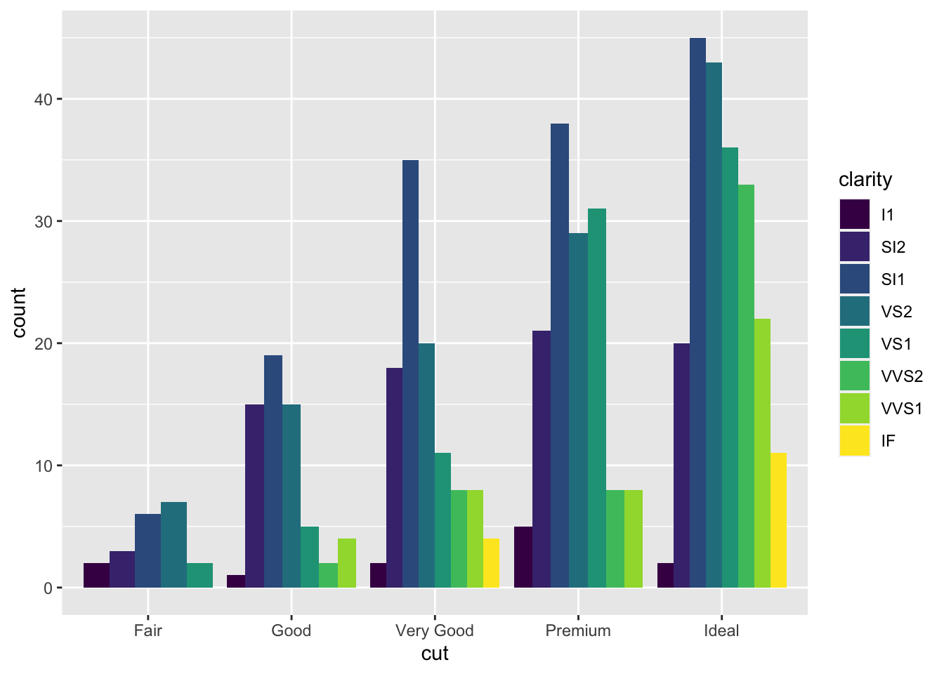
The option position = "fill" is similar to stacking but each set of stacked bars has the same height (corresponding to 100%); this makes the comparison between groups easier. The option position = "dodge" places the rectangles side by side.

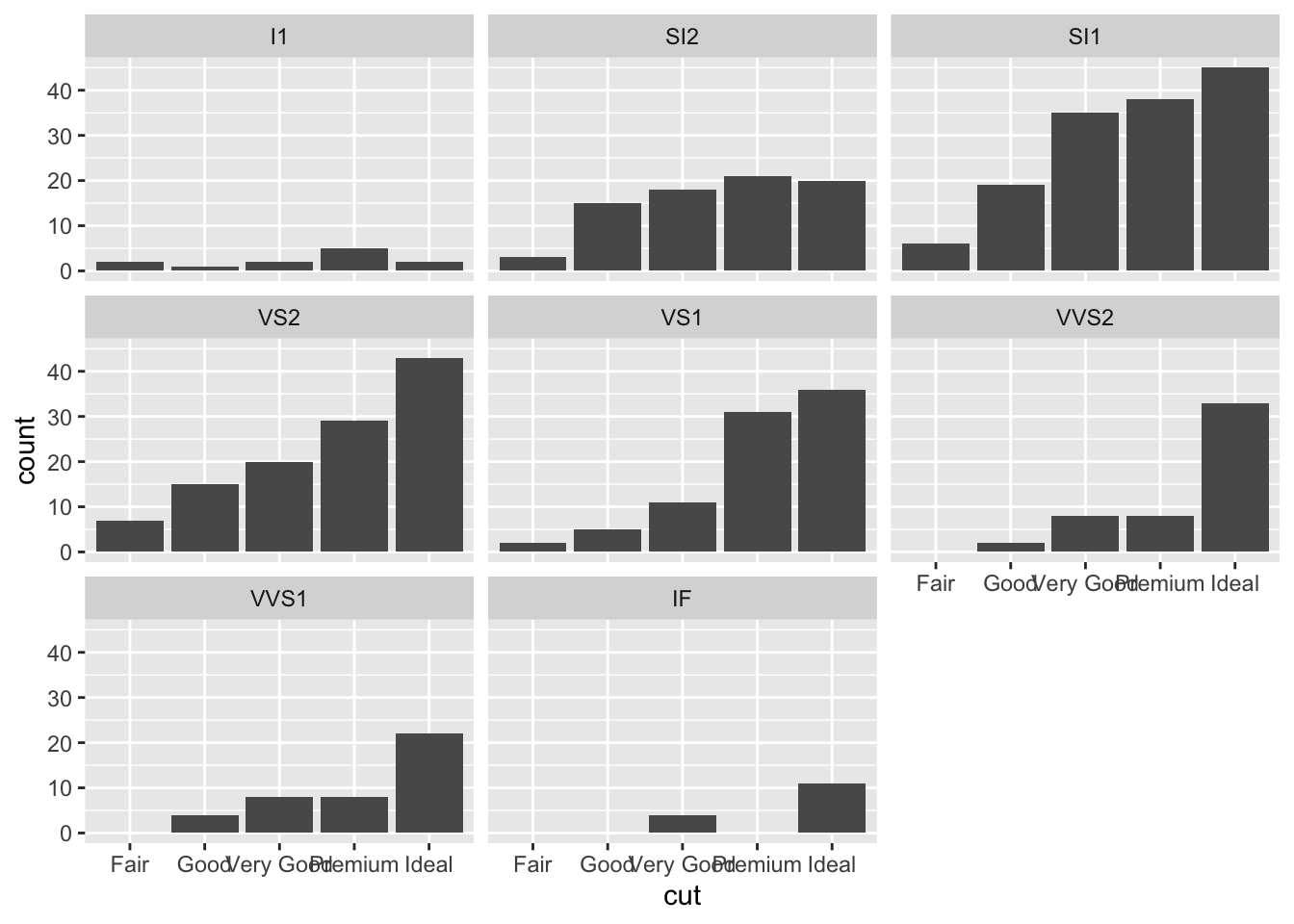
An alternative consists in the use of facet_wrap that will create 8 separate plots (as the number of categories of clarity) each representing the conditional cut distribution:

mydiamonds %>% 
  ggplot() +
  geom_bar(aes(x=cut)) +
  facet_wrap(~clarity)

7.7 Exercises Lecture 4 and 5

7.7.1 Exercise 1

Write the code for the following operations:

Simulate a vector of 15 values from the continuous Uniform distribution defined between 0 and 10 (see ?runif). Set the seed equal to 99.
Round the numbers in the vector to two digits.
Sort the values in the vector in descending order (see ?sort)
Display a few of the largest values with head().

Use both the standard R programming approach and the more modern approach based on the use of the pipe %>% (remember to load the tidyverse library).

7.7.2 Exercise 2

Consider the mtcars data set which is avalaible in R. Type the following code to explore the variables included in the data set (for an explanation of the variables see ?mtcars:

library(tidyverse)
glimpse(mtcars)

## Rows: 32
## Columns: 11
## $ mpg  <dbl> 21.0, 21.0, 22.8, 21.4, 18.7, 18.1, 14.3, 24.4, 22.8, 19.2, 17.8,…
## $ cyl  <dbl> 6, 6, 4, 6, 8, 6, 8, 4, 4, 6, 6, 8, 8, 8, 8, 8, 8, 4, 4, 4, 4, 8,…
## $ disp <dbl> 160.0, 160.0, 108.0, 258.0, 360.0, 225.0, 360.0, 146.7, 140.8, 16…
## $ hp   <dbl> 110, 110, 93, 110, 175, 105, 245, 62, 95, 123, 123, 180, 180, 180…
## $ drat <dbl> 3.90, 3.90, 3.85, 3.08, 3.15, 2.76, 3.21, 3.69, 3.92, 3.92, 3.92,…
## $ wt   <dbl> 2.620, 2.875, 2.320, 3.215, 3.440, 3.460, 3.570, 3.190, 3.150, 3.…
## $ qsec <dbl> 16.46, 17.02, 18.61, 19.44, 17.02, 20.22, 15.84, 20.00, 22.90, 18…
## $ vs   <dbl> 0, 0, 1, 1, 0, 1, 0, 1, 1, 1, 1, 0, 0, 0, 0, 0, 0, 1, 1, 1, 1, 0,…
## $ am   <dbl> 1, 1, 1, 0, 0, 0, 0, 0, 0, 0, 0, 0, 0, 0, 0, 0, 0, 1, 1, 1, 0, 0,…
## $ gear <dbl> 4, 4, 4, 3, 3, 3, 3, 4, 4, 4, 4, 3, 3, 3, 3, 3, 3, 4, 4, 4, 3, 3,…
## $ carb <dbl> 4, 4, 1, 1, 2, 1, 4, 2, 2, 4, 4, 3, 3, 3, 4, 4, 4, 1, 2, 1, 1, 2,…

Use the following code to create a new variable named car_model that contains the names of the cars, now available as row names.

mtcars = mtcars %>%
        rownames_to_column("car_model")
glimpse(mtcars)

## Rows: 32
## Columns: 12
## $ car_model <chr> "Mazda RX4", "Mazda RX4 Wag", "Datsun 710", "Hornet 4 Drive"…
## $ mpg       <dbl> 21.0, 21.0, 22.8, 21.4, 18.7, 18.1, 14.3, 24.4, 22.8, 19.2, …
## $ cyl       <dbl> 6, 6, 4, 6, 8, 6, 8, 4, 4, 6, 6, 8, 8, 8, 8, 8, 8, 4, 4, 4, …
## $ disp      <dbl> 160.0, 160.0, 108.0, 258.0, 360.0, 225.0, 360.0, 146.7, 140.…
## $ hp        <dbl> 110, 110, 93, 110, 175, 105, 245, 62, 95, 123, 123, 180, 180…
## $ drat      <dbl> 3.90, 3.90, 3.85, 3.08, 3.15, 2.76, 3.21, 3.69, 3.92, 3.92, …
## $ wt        <dbl> 2.620, 2.875, 2.320, 3.215, 3.440, 3.460, 3.570, 3.190, 3.15…
## $ qsec      <dbl> 16.46, 17.02, 18.61, 19.44, 17.02, 20.22, 15.84, 20.00, 22.9…
## $ vs        <dbl> 0, 0, 1, 1, 0, 1, 0, 1, 1, 1, 1, 0, 0, 0, 0, 0, 0, 1, 1, 1, …
## $ am        <dbl> 1, 1, 1, 0, 0, 0, 0, 0, 0, 0, 0, 0, 0, 0, 0, 0, 0, 1, 1, 1, …
## $ gear      <dbl> 4, 4, 4, 3, 3, 3, 3, 4, 4, 4, 4, 3, 3, 3, 3, 3, 3, 4, 4, 4, …
## $ carb      <dbl> 4, 4, 1, 1, 2, 1, 4, 2, 2, 4, 4, 3, 3, 3, 4, 4, 4, 1, 2, 1, …

Use the following code to define two factors for cyl and am which are now considered as dbl variables:

mtcars$cyl = factor(mtcars$cyl)
mtcars$am = factor(mtcars$am,labels=c("automatic","manual"))

How many observations and variables are available?
Print (on the screen) the hp variable using the select() function. Try also to use the pull() function. Which is the difference?
Print out all but the hp column using the select() function.
Print out the following variables: mpg, hp, vs, am, gear. Suggestion: use : if necessary.
Provide the frequency distribution (absolute, relative and percentage) for the am variable (transmission).
Consider the variables wt (weight) and mpg (miles/gallon). By using plot() and then ggplot() produce the scatterplot which displays consumption as a function of weight. Which kind of relationship does exist between the two variables?
Consider the ggplot code used for the previous sub-exercise. Plot the same variables but use the variable am (transmission) to color the points. Comment the plot.
Create a new variable km_per_litre using the mutate() function. Suggestion: 1 mpg is 0.425 km/l. Save the variable in the dataframe. Provide the average value of km_per_litre conditioning on am (transmission). For which kind of transmission is the average fuel consumption higher?
Reorder the observations so that you can easily find the car with the lowest consumption.
Select all the observations which have mpg>20 and hp>100 and compute the average for the km_per_litre variable.
Compute the distribution (absolute frequencies) of the car by gear. Moreover, compute the mean consumption (mpg) conditionally on the gear.
Create a new variable named performance given by hp/mpg. Filter the first 10 best cars in terms of performance (suggestion: use the function top_n).
Display hp (gross horsepower) as a function of cyl by using ggplot(). Use facet_wrap to produce different plots according to am (transmisison). Which kind of relationship does exist between the two variables?

7.7.3 Exercise 3

Consider the iris dataset available in R. It contains the measurements in centimeters of the variables sepal length and width and petal length and width, respectively, for some flowers from each of 3 species of iris. See ?iris.

glimpse(iris)

## Rows: 150
## Columns: 5
## $ Sepal.Length <dbl> 5.1, 4.9, 4.7, 4.6, 5.0, 5.4, 4.6, 5.0, 4.4, 4.9, 5.4, 4.…
## $ Sepal.Width  <dbl> 3.5, 3.0, 3.2, 3.1, 3.6, 3.9, 3.4, 3.4, 2.9, 3.1, 3.7, 3.…
## $ Petal.Length <dbl> 1.4, 1.4, 1.3, 1.5, 1.4, 1.7, 1.4, 1.5, 1.4, 1.5, 1.5, 1.…
## $ Petal.Width  <dbl> 0.2, 0.2, 0.2, 0.2, 0.2, 0.4, 0.3, 0.2, 0.2, 0.1, 0.2, 0.…
## $ Species      <fct> setosa, setosa, setosa, setosa, setosa, setosa, setosa, s…

Compute the frequency distribution (absolute, relative and percentage frequencies) of Species. Which are the available species?
Compute the average and the standard deviation for all the numeric column of iris. Then compute the same statistics by conditioning on species. Suggestion: use the function summarise_if (see ?summarise_if, in this case test if the column is.numeric):
Compute the average of Sepal.Length and Petal.Length by Species. Which is the species with the highest average sepal/petal length?
Plot Petal.Width as a function of Petal.Length with a scatterplot. Use the species for the color and shape of the points. Which kind of relationship does it exist?
Add to the data frame a new variable called Ratio.Sepal which is given by Sepal.Length/Petal.Width. Compute the mode of this variable (by computing the frequency distribution and then reordering by the frequencies).

7.7.4 Exercise 4

Consider the data available in the fev.csv file (use fevdata as the name of the dataframe). The dataset examines if respiratory function in children was influenced by exposure to smoking at home. The included variables are:

Age
FEV: forced expiratory volume in liters (lung capacity)
Ht: height measured in inches
Gender: 0=female, 1=male
Smoke: exposure to smoking (0=no, 1=yes)

Import the data in R and check the type of variables contained in the dataframe.
Trasform Gender and Smoke into factors.
Compute the univariate and bivariate contingency table (with percentage frequencies) for the new factors Gender and Smoke.
Represent graphically height, age and FEV by histogram or barplot. Avoid using count on the y-axis. Comment the plots.
Using boxplots study the distribution of Age and then Ht conditioned on Gender. Comment the plots.
Using a scatterplot represent FEV as a function of Ht. Use different colors according to the smoke information. Comment.
Produce different scatterplots representing FEV as a function of Ht according to the gender categories. Include also in the plots a smooth line. Comment the plots.

7.7.5 Exercise 5

Consider the Titanic data contained in the file titanic_tr.csv. This is a subset (with 891 observations and 11 variables) of the original dataset. The included variables are the following:

pclass: passenger class (first, second or third)
survived: survived (1) or died (0)
name: passenger name
sex: passenger sex
age: passenger age
sibSp: number of siblings/spouses aboard
parch: number of parents/children aboard
ticket: ticket number
fare: fare (cost of the ticket)
cabin: cabin id
embarked: port of embarkation (S = Southampton, C = Cherbourg, Q = Queenstown)

Import the data and explore them. Transform the variable survived, pclass and sex into factors.
Represent graphically the distribution of the variable fare. Moreover, compute the average ticket price paid by passengers. Finally, compute the percentage of tickets paid more than 100$.
Represent graphically the distribution of the variable age. Compute the average age. Pay attention to missing values. Consider the possibility of using the na.rm option of the function mean (see ?mean).
Study the distribution of sex by using a barplot. Derive also the corresponding table frequency distribution.
By using a graphical representation study the distribution of age conditionally on gender. Moreover, compute the mean age by gender.
Compute the (absolute and percentage) bivariate distribution of sex and survived (percentages should be computed with respect to the total sample size). Moreover, produce the corresponding plot which represents the two factors.
Derive the percentage distribution of survived conditioned on sex. Produce also the corresponding plot.
Filter by sex and consider only males and compute the frequency distribution of the variable embarked. Produce the corresponding plot.
Create a new variable called agecat with two categories (minor if age < 18, major otherwise). Then derive the frequency distribution of agecat.
Produce a scatterplot with age on the x-axis and fare on the y-axis. Use a different point color according to gender.
Study the relationship between age and fare, as you did in the previous sub-exercise, producing sub-plots according to embarked.