6 Lecture 4 - 21/12/2020

In this lecture we will learn another R programming approach based on the tidyverse package. This is alternative to the base R code we learnt in the first lectures.

6.1 Tidyverse

Tidyverse is a collection of R packages designed for data science (see Figure 6.1. All the packages share an underlying design philosophy, grammar, and data structures. See here for more details.

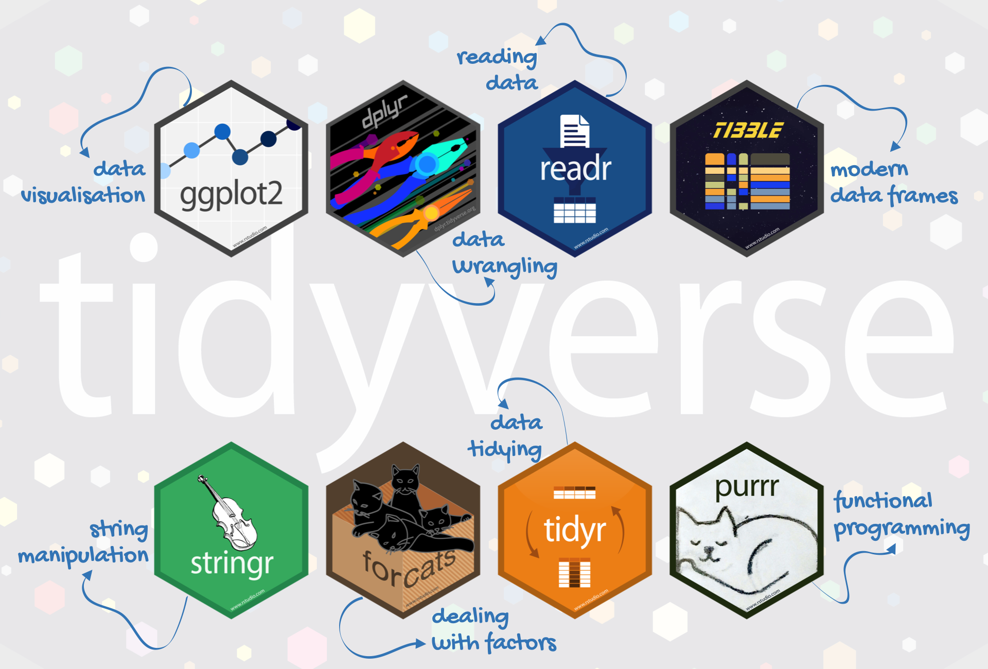
Figure 6.1: Packages included in tidyverse

The tidyverse-based functions process faster than base R functions. It is because they are written in a computationally efficient manner and are also more stable in the syntax and better supports data frames than vectors.

library(tidyverse)

## ── Attaching packages ─────────────────────────────────────── tidyverse 1.3.0 ──

## ✓ ggplot2 3.3.3     ✓ purrr   0.3.4
## ✓ tibble  3.1.0     ✓ dplyr   1.0.5
## ✓ tidyr   1.1.3     ✓ stringr 1.4.0
## ✓ readr   1.3.1     ✓ forcats 0.5.0

## ── Conflicts ────────────────────────────────────────── tidyverse_conflicts() ──
## x dplyr::filter() masks stats::filter()
## x dplyr::lag()    masks stats::lag()

6.2 The pipe operator

Let’s consider a general R function named f with argument x. We usually use the following approach when we need to apply f:

f(x)

An alternative is given by the pipe operator %>% which is part of the dplyr package (see here for more details). It works as follows

x %>% f() 
#this is equivalent to f(x)

Basically, the pipe tells R to pass x as the first argument of the function f. The shortcut to type the pipe operator in RStudio is given by CTRL/CMD + Shift + M.

We simulate a sample of data in order to run some simple examples with the pipe operator. By using the function sample we draw randomly (without replacement) 5 numbers between 1 and 20 (1:20).

set.seed(44)
x = sample(1:20, 5)
x

## [1] 17 11  1 20  5

We are now interested in computing the log transformation of the vector x. By adopting the standard R programming we would use:

log(x)

## [1] 2.833213 2.397895 0.000000 2.995732 1.609438

while with the pipe operator we have

x %>% log()

## [1] 2.833213 2.397895 0.000000 2.995732 1.609438

#it's also possible to omit the parentheses given that there is no input

where x is taken as the first argument of the function log. It is also possible to include other arguments, such as for example the base of the logarithm (in this case equal to 5). In this case note that x %>% f(y) is equivalent to f(x,y).

#standard programming
log(x, base=5)

## [1] 1.760374 1.489896 0.000000 1.861353 1.000000

#pipe based programming
x %>% log(base=5)

## [1] 1.760374 1.489896 0.000000 1.861353 1.000000

We want now to apply the log transformation and then round the corresponding output to 2 digits. This requires the use of two functions (log and round). In general, when we apply 3 functions (f and then g and finally h), we have that x %>% f %>% g %>% h is equivalent to h(g(f(x))).

# standard programming
round(log(x), 2)

## [1] 2.83 2.40 0.00 3.00 1.61

# pipe based programming
x %>%  log %>% round(2)

## [1] 2.83 2.40 0.00 3.00 1.61

We now add a new function: after rounding the log output we compute the sum of the 5 numbers

# standard programming
sum(round(log(x),2))

## [1] 9.84

# pipe based programming
x %>% log %>% round(2) %>% sum 

## [1] 9.84

We want now to use the sum result as the base of the log transformation of the number 5

# standard programming
log(5, base = sum(round(log(x),2)))

## [1] 0.7039008

# pipe based programming
x %>% log %>% round(2) %>% sum %>% log(5,base=.) 

## [1] 0.7039008

The symbol . is the placeholder and is used when the output of the previous pipe should not be used as the first input of the following function. In general, x %>% f(y, z = .) is equivalent to f(y, z = x).

When it is not convenient to use the pipe:

• when the pipes are longer than 10 steps. In this case the suggestion is to create intermediate objects with meaningful names (that can help understanding what the code does;
• when you have multiple inputs or outputs (e.g. when there is no primary object being transformed but two or more objects being combined together).

6.3 dyplyr verbs

dplyr is a grammar of data manipulation, providing a consistent set of verbs that help you solve the most common data manipulation challenges: - select: pick variables (columns) based on their names - filter pick observations (rows) based on their values - mutate: add new variables that are functions of existing variables - summarise: reduce multiple values down to a single summary (e.g. mean) - arrange: change the ordering of the rows

All verbs work similarly: - the first argument is a data frame; - the subsequent arguments describe what to do with the data frame using the variable names (without quotes); - the result is a new data frame.

In the following we will take into account all the dplyr verbs by considering the diamonds dataset which contains the prices and other attributes of almost 54,000 diamonds (see ?diamonds). If we use the function class to understand the nature of diamonds we get the following output:

class(diamonds)

## [1] "tbl_df"     "tbl"        "data.frame"

The term tbl (tibble) is the tidyverse version of a classical R data frame. Tiblles are very similar to data frame (they just contain/display more information) and are designed to be used with the tidyverse syntax style.

To get the list and the type of variables included in diamonds we can use the standard str or the corresponding tidyverse function named glimpse:

str(diamonds)

## tibble[,10] [53,940 × 10] (S3: tbl_df/tbl/data.frame)
##  $ carat  : num [1:53940] 0.23 0.21 0.23 0.29 0.31 0.24 0.24 0.26 0.22 0.23 ...
##  $ cut    : Ord.factor w/ 5 levels "Fair"<"Good"<..: 5 4 2 4 2 3 3 3 1 3 ...
##  $ color  : Ord.factor w/ 7 levels "D"<"E"<"F"<"G"<..: 2 2 2 6 7 7 6 5 2 5 ...
##  $ clarity: Ord.factor w/ 8 levels "I1"<"SI2"<"SI1"<..: 2 3 5 4 2 6 7 3 4 5 ...
##  $ depth  : num [1:53940] 61.5 59.8 56.9 62.4 63.3 62.8 62.3 61.9 65.1 59.4 ...
##  $ table  : num [1:53940] 55 61 65 58 58 57 57 55 61 61 ...
##  $ price  : int [1:53940] 326 326 327 334 335 336 336 337 337 338 ...
##  $ x      : num [1:53940] 3.95 3.89 4.05 4.2 4.34 3.94 3.95 4.07 3.87 4 ...
##  $ y      : num [1:53940] 3.98 3.84 4.07 4.23 4.35 3.96 3.98 4.11 3.78 4.05 ...
##  $ z      : num [1:53940] 2.43 2.31 2.31 2.63 2.75 2.48 2.47 2.53 2.49 2.39 ...

glimpse(diamonds)

## Rows: 53,940
## Columns: 10
## $ carat   <dbl> 0.23, 0.21, 0.23, 0.29, 0.31, 0.24, 0.24, 0.26, 0.22, 0.23, 0.…
## $ cut     <ord> Ideal, Premium, Good, Premium, Good, Very Good, Very Good, Ver…
## $ color   <ord> E, E, E, I, J, J, I, H, E, H, J, J, F, J, E, E, I, J, J, J, I,…
## $ clarity <ord> SI2, SI1, VS1, VS2, SI2, VVS2, VVS1, SI1, VS2, VS1, SI1, VS1, …
## $ depth   <dbl> 61.5, 59.8, 56.9, 62.4, 63.3, 62.8, 62.3, 61.9, 65.1, 59.4, 64…
## $ table   <dbl> 55, 61, 65, 58, 58, 57, 57, 55, 61, 61, 55, 56, 61, 54, 62, 58…
## $ price   <int> 326, 326, 327, 334, 335, 336, 336, 337, 337, 338, 339, 340, 34…
## $ x       <dbl> 3.95, 3.89, 4.05, 4.20, 4.34, 3.94, 3.95, 4.07, 3.87, 4.00, 4.…
## $ y       <dbl> 3.98, 3.84, 4.07, 4.23, 4.35, 3.96, 3.98, 4.11, 3.78, 4.05, 4.…
## $ z       <dbl> 2.43, 2.31, 2.31, 2.63, 2.75, 2.48, 2.47, 2.53, 2.49, 2.39, 2.…

6.3.1 Verb 1: select

This verb is used to select some of the columns by name. For example, to select the variable named carat we use the following code:

diamonds %>% select(carat) 

## # A tibble: 53,940 x 1
##    carat
##    <dbl>
##  1  0.23
##  2  0.21
##  3  0.23
##  4  0.29
##  5  0.31
##  6  0.24
##  7  0.24
##  8  0.26
##  9  0.22
## 10  0.23
## # … with 53,930 more rows

Selecting more than one column is very simple:

diamonds %>% select(carat, cut, color, price)

## # A tibble: 53,940 x 4
##    carat cut       color price
##    <dbl> <ord>     <ord> <int>
##  1  0.23 Ideal     E       326
##  2  0.21 Premium   E       326
##  3  0.23 Good      E       327
##  4  0.29 Premium   I       334
##  5  0.31 Good      J       335
##  6  0.24 Very Good J       336
##  7  0.24 Very Good I       336
##  8  0.26 Very Good H       337
##  9  0.22 Fair      E       337
## 10  0.23 Very Good H       338
## # … with 53,930 more rows

Given that carat, cut and color are consecutive, the following code is also possible:

diamonds %>% select(carat : color, price)

## # A tibble: 53,940 x 4
##    carat cut       color price
##    <dbl> <ord>     <ord> <int>
##  1  0.23 Ideal     E       326
##  2  0.21 Premium   E       326
##  3  0.23 Good      E       327
##  4  0.29 Premium   I       334
##  5  0.31 Good      J       335
##  6  0.24 Very Good J       336
##  7  0.24 Very Good I       336
##  8  0.26 Very Good H       337
##  9  0.22 Fair      E       337
## 10  0.23 Very Good H       338
## # … with 53,930 more rows

Moreover, it is also possible to select all the columns whose name starts with the letter “c” by using starts_with combined with the select function:

diamonds %>% select(starts_with("c"))

## # A tibble: 53,940 x 4
##    carat cut       color clarity
##    <dbl> <ord>     <ord> <ord>  
##  1  0.23 Ideal     E     SI2    
##  2  0.21 Premium   E     SI1    
##  3  0.23 Good      E     VS1    
##  4  0.29 Premium   I     VS2    
##  5  0.31 Good      J     SI2    
##  6  0.24 Very Good J     VVS2   
##  7  0.24 Very Good I     VVS1   
##  8  0.26 Very Good H     SI1    
##  9  0.22 Fair      E     VS2    
## 10  0.23 Very Good H     VS1    
## # … with 53,930 more rows

It is also possible to specify a criterion which excludes from the selection some variables. For example, to select all the columns but carat we use the - symbol:

diamonds %>% select(-carat)

## # A tibble: 53,940 x 9
##    cut       color clarity depth table price     x     y     z
##    <ord>     <ord> <ord>   <dbl> <dbl> <int> <dbl> <dbl> <dbl>
##  1 Ideal     E     SI2      61.5    55   326  3.95  3.98  2.43
##  2 Premium   E     SI1      59.8    61   326  3.89  3.84  2.31
##  3 Good      E     VS1      56.9    65   327  4.05  4.07  2.31
##  4 Premium   I     VS2      62.4    58   334  4.2   4.23  2.63
##  5 Good      J     SI2      63.3    58   335  4.34  4.35  2.75
##  6 Very Good J     VVS2     62.8    57   336  3.94  3.96  2.48
##  7 Very Good I     VVS1     62.3    57   336  3.95  3.98  2.47
##  8 Very Good H     SI1      61.9    55   337  4.07  4.11  2.53
##  9 Fair      E     VS2      65.1    61   337  3.87  3.78  2.49
## 10 Very Good H     VS1      59.4    61   338  4     4.05  2.39
## # … with 53,930 more rows

We proceed similarly to select all the columns but not the ones with a name starting with “c”:

diamonds %>% select(- starts_with("c"))

## # A tibble: 53,940 x 6
##    depth table price     x     y     z
##    <dbl> <dbl> <int> <dbl> <dbl> <dbl>
##  1  61.5    55   326  3.95  3.98  2.43
##  2  59.8    61   326  3.89  3.84  2.31
##  3  56.9    65   327  4.05  4.07  2.31
##  4  62.4    58   334  4.2   4.23  2.63
##  5  63.3    58   335  4.34  4.35  2.75
##  6  62.8    57   336  3.94  3.96  2.48
##  7  62.3    57   336  3.95  3.98  2.47
##  8  61.9    55   337  4.07  4.11  2.53
##  9  65.1    61   337  3.87  3.78  2.49
## 10  59.4    61   338  4     4.05  2.39
## # … with 53,930 more rows

6.3.2 Verb 2: filter

The verb filter can be used to select the observations satisfying some criterion. Consider the example the selection of the diamonds with variable cut equal to the category “Premium”:

diamonds %>% filter(cut == "Premium")

## # A tibble: 13,791 x 10
##    carat cut     color clarity depth table price     x     y     z
##    <dbl> <ord>   <ord> <ord>   <dbl> <dbl> <int> <dbl> <dbl> <dbl>
##  1  0.21 Premium E     SI1      59.8    61   326  3.89  3.84  2.31
##  2  0.29 Premium I     VS2      62.4    58   334  4.2   4.23  2.63
##  3  0.22 Premium F     SI1      60.4    61   342  3.88  3.84  2.33
##  4  0.2  Premium E     SI2      60.2    62   345  3.79  3.75  2.27
##  5  0.32 Premium E     I1       60.9    58   345  4.38  4.42  2.68
##  6  0.24 Premium I     VS1      62.5    57   355  3.97  3.94  2.47
##  7  0.29 Premium F     SI1      62.4    58   403  4.24  4.26  2.65
##  8  0.22 Premium E     VS2      61.6    58   404  3.93  3.89  2.41
##  9  0.22 Premium D     VS2      59.3    62   404  3.91  3.88  2.31
## 10  0.3  Premium J     SI2      59.3    61   405  4.43  4.38  2.61
## # … with 13,781 more rows

It is also possible to include more conditions. Select for example the diamonds with cut equal to “Premium” AND color equal to “D” (the AND can be specified by using & or comma):

diamonds %>% filter(cut == "Premium" & color == "D") 

## # A tibble: 1,603 x 10
##    carat cut     color clarity depth table price     x     y     z
##    <dbl> <ord>   <ord> <ord>   <dbl> <dbl> <int> <dbl> <dbl> <dbl>
##  1  0.22 Premium D     VS2      59.3    62   404  3.91  3.88  2.31
##  2  0.3  Premium D     SI1      62.6    59   552  4.23  4.27  2.66
##  3  0.71 Premium D     SI2      61.7    59  2768  5.71  5.67  3.51
##  4  0.71 Premium D     VS2      62.5    60  2770  5.65  5.61  3.52
##  5  0.7  Premium D     VS2      58      62  2773  5.87  5.78  3.38
##  6  0.72 Premium D     SI1      62.7    59  2782  5.73  5.69  3.58
##  7  0.7  Premium D     SI1      62.8    60  2782  5.68  5.66  3.56
##  8  0.72 Premium D     SI2      62      60  2795  5.73  5.69  3.54
##  9  0.71 Premium D     SI1      62.7    60  2797  5.67  5.71  3.57
## 10  0.71 Premium D     SI1      61.3    58  2797  5.73  5.75  3.52
## # … with 1,593 more rows

diamonds %>% filter(cut == "Premium" , color == "D") 

## # A tibble: 1,603 x 10
##    carat cut     color clarity depth table price     x     y     z
##    <dbl> <ord>   <ord> <ord>   <dbl> <dbl> <int> <dbl> <dbl> <dbl>
##  1  0.22 Premium D     VS2      59.3    62   404  3.91  3.88  2.31
##  2  0.3  Premium D     SI1      62.6    59   552  4.23  4.27  2.66
##  3  0.71 Premium D     SI2      61.7    59  2768  5.71  5.67  3.51
##  4  0.71 Premium D     VS2      62.5    60  2770  5.65  5.61  3.52
##  5  0.7  Premium D     VS2      58      62  2773  5.87  5.78  3.38
##  6  0.72 Premium D     SI1      62.7    59  2782  5.73  5.69  3.58
##  7  0.7  Premium D     SI1      62.8    60  2782  5.68  5.66  3.56
##  8  0.72 Premium D     SI2      62      60  2795  5.73  5.69  3.54
##  9  0.71 Premium D     SI1      62.7    60  2797  5.67  5.71  3.57
## 10  0.71 Premium D     SI1      61.3    58  2797  5.73  5.75  3.52
## # … with 1,593 more rows

If we are interested in filtering th diamonds with a price between 500 and 600 dollars the following two alternative codes can be adopted:

diamonds %>% filter(price > 500 & price < 600)

## # A tibble: 2,360 x 10
##    carat cut       color clarity depth table price     x     y     z
##    <dbl> <ord>     <ord> <ord>   <dbl> <dbl> <int> <dbl> <dbl> <dbl>
##  1  0.35 Ideal     I     VS1      60.9  57     552  4.54  4.59  2.78
##  2  0.3  Premium   D     SI1      62.6  59     552  4.23  4.27  2.66
##  3  0.3  Ideal     D     SI1      62.5  57     552  4.29  4.32  2.69
##  4  0.3  Ideal     D     SI1      62.1  56     552  4.3   4.33  2.68
##  5  0.42 Premium   I     SI2      61.5  59     552  4.78  4.84  2.96
##  6  0.28 Ideal     G     VVS2     61.4  56     553  4.19  4.22  2.58
##  7  0.32 Ideal     I     VVS1     62    55.3   553  4.39  4.42  2.73
##  8  0.31 Very Good G     SI1      63.3  57     553  4.33  4.3   2.73
##  9  0.31 Premium   G     SI1      61.8  58     553  4.35  4.32  2.68
## 10  0.24 Premium   E     VVS1     60.7  58     553  4.01  4.03  2.44
## # … with 2,350 more rows

diamonds %>% filter(between(price, 500,600))

## # A tibble: 2,407 x 10
##    carat cut       color clarity depth table price     x     y     z
##    <dbl> <ord>     <ord> <ord>   <dbl> <dbl> <int> <dbl> <dbl> <dbl>
##  1  0.35 Ideal     I     VS1      60.9  57     552  4.54  4.59  2.78
##  2  0.3  Premium   D     SI1      62.6  59     552  4.23  4.27  2.66
##  3  0.3  Ideal     D     SI1      62.5  57     552  4.29  4.32  2.69
##  4  0.3  Ideal     D     SI1      62.1  56     552  4.3   4.33  2.68
##  5  0.42 Premium   I     SI2      61.5  59     552  4.78  4.84  2.96
##  6  0.28 Ideal     G     VVS2     61.4  56     553  4.19  4.22  2.58
##  7  0.32 Ideal     I     VVS1     62    55.3   553  4.39  4.42  2.73
##  8  0.31 Very Good G     SI1      63.3  57     553  4.33  4.3   2.73
##  9  0.31 Premium   G     SI1      61.8  58     553  4.35  4.32  2.68
## 10  0.24 Premium   E     VVS1     60.7  58     553  4.01  4.03  2.44
## # … with 2,397 more rows

The output of a selection can be saved in a new data frame as follows:

myselection = diamonds %>% filter(between(price, 500,600))

To select diamonds with cut equal to fair OR good we can use the | operator or the %in% function:

diamonds %>% filter(cut=="Fair" | cut=="Good")

## # A tibble: 6,516 x 10
##    carat cut   color clarity depth table price     x     y     z
##    <dbl> <ord> <ord> <ord>   <dbl> <dbl> <int> <dbl> <dbl> <dbl>
##  1  0.23 Good  E     VS1      56.9    65   327  4.05  4.07  2.31
##  2  0.31 Good  J     SI2      63.3    58   335  4.34  4.35  2.75
##  3  0.22 Fair  E     VS2      65.1    61   337  3.87  3.78  2.49
##  4  0.3  Good  J     SI1      64      55   339  4.25  4.28  2.73
##  5  0.3  Good  J     SI1      63.4    54   351  4.23  4.29  2.7 
##  6  0.3  Good  J     SI1      63.8    56   351  4.23  4.26  2.71
##  7  0.3  Good  I     SI2      63.3    56   351  4.26  4.3   2.71
##  8  0.23 Good  F     VS1      58.2    59   402  4.06  4.08  2.37
##  9  0.23 Good  E     VS1      64.1    59   402  3.83  3.85  2.46
## 10  0.31 Good  H     SI1      64      54   402  4.29  4.31  2.75
## # … with 6,506 more rows

diamonds %>% filter(cut %in% c("Fair","Good"))

## # A tibble: 6,516 x 10
##    carat cut   color clarity depth table price     x     y     z
##    <dbl> <ord> <ord> <ord>   <dbl> <dbl> <int> <dbl> <dbl> <dbl>
##  1  0.23 Good  E     VS1      56.9    65   327  4.05  4.07  2.31
##  2  0.31 Good  J     SI2      63.3    58   335  4.34  4.35  2.75
##  3  0.22 Fair  E     VS2      65.1    61   337  3.87  3.78  2.49
##  4  0.3  Good  J     SI1      64      55   339  4.25  4.28  2.73
##  5  0.3  Good  J     SI1      63.4    54   351  4.23  4.29  2.7 
##  6  0.3  Good  J     SI1      63.8    56   351  4.23  4.26  2.71
##  7  0.3  Good  I     SI2      63.3    56   351  4.26  4.3   2.71
##  8  0.23 Good  F     VS1      58.2    59   402  4.06  4.08  2.37
##  9  0.23 Good  E     VS1      64.1    59   402  3.83  3.85  2.46
## 10  0.31 Good  H     SI1      64      54   402  4.29  4.31  2.75
## # … with 6,506 more rows

The code diamonds %>% filter(cut == c("Fair","Good")) does not perform what we mean to do. For an interesting discussion about the difference between == and %in% see here.

6.3.3 Verb 4: summarise

This verbs can be used to compute summary statistics. For example the following code computes the mean and median of price.

diamonds %>% 
  summarise(mean(price),
            median(price))

## # A tibble: 1 x 2
##   `mean(price)` `median(price)`
##           <dbl>           <dbl>
## 1         3933.            2401

The output is automatically labelled but it is also possible to specify different labels as follows:

diamonds %>% 
  summarise(mean_price = mean(price),
            median_price = median(price))

## # A tibble: 1 x 2
##   mean_price median_price
##        <dbl>        <dbl>
## 1      3933.         2401

It is also possible to compute how many observations (and its corresponding proportion and percentage) satisfying a certain condition, e.g. the number of diamonds with a price > 15000$:

diamonds %>% 
  summarise(veryexp = sum(price > 15000),
            veryexpprop = mean(price>15000),
            veryexpperc = mean(price>15000)*100)

## # A tibble: 1 x 3
##   veryexp veryexpprop veryexpperc
##     <int>       <dbl>       <dbl>
## 1    1655      0.0307        3.07

It is also interesting to compute summary statistics conditionally on the categories of a qualitative variable (i.e. a factor). This can be done by combining the group_by function with the summarise function. Let’s compute for example the mean, min and max price conditionally on the categories of cut:

diamonds %>% 
  group_by(cut) %>% 
  summarise(mean(price),min(price),max(price))

## # A tibble: 5 x 4
##   cut       `mean(price)` `min(price)` `max(price)`
##   <ord>             <dbl>        <int>        <int>
## 1 Fair              4359.          337        18574
## 2 Good              3929.          327        18788
## 3 Very Good         3982.          336        18818
## 4 Premium           4584.          326        18823
## 5 Ideal             3458.          326        18806

In particular, group_by splits the original data set into different groups and for each of them the requested summary statistics are computed. In this case we obtain 5 values of the mean, min and max price according to the number of categories of the variable cut. It is also possible to condition on two different factors, such as for example cut and color:

diamonds %>% 
  group_by(cut,color) %>% 
  summarise(mean(price)) 

## `summarise()` has grouped output by 'cut'. You can override using the `.groups` argument.

## # A tibble: 35 x 3
## # Groups:   cut [5]
##    cut   color `mean(price)`
##    <ord> <ord>         <dbl>
##  1 Fair  D             4291.
##  2 Fair  E             3682.
##  3 Fair  F             3827.
##  4 Fair  G             4239.
##  5 Fair  H             5136.
##  6 Fair  I             4685.
##  7 Fair  J             4976.
##  8 Good  D             3405.
##  9 Good  E             3424.
## 10 Good  F             3496.
## # … with 25 more rows

In this case each category of cut is combined with each category of color and then the mean price is computed.

The function group_by can by combined with summarise also to compute frequency distribution, by means of the n() function which gives the current group size:

diamonds %>% 
  group_by(cut) %>% 
  summarise(AbsFreq = n())

## # A tibble: 5 x 2
##   cut       AbsFreq
##   <ord>       <int>
## 1 Fair         1610
## 2 Good         4906
## 3 Very Good   12082
## 4 Premium     13791
## 5 Ideal       21551

This is an alternative to the table standard function introduced in Lecture 3:

table(diamonds$cut)

## 
##      Fair      Good Very Good   Premium     Ideal 
##      1610      4906     12082     13791     21551

Similarly, percentages can be easily computed by using AbsFreq which are quantities available for new computations:

diamonds %>% 
  group_by(cut) %>% 
  summarise(AbsFreq = n(), Perc = AbsFreq/nrow(diamonds)*100)

## # A tibble: 5 x 3
##   cut       AbsFreq  Perc
##   <ord>       <int> <dbl>
## 1 Fair         1610  2.98
## 2 Good         4906  9.10
## 3 Very Good   12082 22.4 
## 4 Premium     13791 25.6 
## 5 Ideal       21551 40.0

A shorter alternative for computing the frequency table si given by the count function which let you quickly count the unique values of one or more variables. Basically, df %>% count(a, b) is roughly equivalent to df %>% group_by(a, b) %>% summarise(n = n()). Here below we have an example:

diamonds %>% 
  count(cut)

## # A tibble: 5 x 2
##   cut           n
##   <ord>     <int>
## 1 Fair       1610
## 2 Good       4906
## 3 Very Good 12082
## 4 Premium   13791
## 5 Ideal     21551

6.3.4 Verb 5: mutate

The verb mutate can be used to create new column in the data frame. For example, let’s create a new column given by a categorical variables with two categories: “Yes” if the price is < 1000$, “No” otherwise. For doing this we will make use of the ifelse function, already introduced during Lecture 2. We will call the new column as newcol and will save the new data frame (with one more column) in a new object named newdiamonds:

newdiamonds = diamonds %>% 
  mutate(newcol = ifelse(price < 1000, "Yes", "No"))

To derive the frequency distribution of newcol we proceed as described above, computing also percentages by means of mutate:

newdiamonds %>% 
  count(newcol) %>% 
  #summarise(perc=n/nrow(newdiamonds)*100)
  mutate(perc=n/nrow(newdiamonds)*100)

## # A tibble: 2 x 3
##   newcol     n  perc
##   <chr>  <int> <dbl>
## 1 No     39441  73.1
## 2 Yes    14499  26.9

6.3.5 Verb 6: arrange

The verb arrange can be used to sort observations with respect to the values of a given variable. For example, we can sort diamonds according to price (by default the ascending order is adopted):

diamonds %>% 
  arrange(price) %>% 
  tail

## # A tibble: 6 x 10
##   carat cut       color clarity depth table price     x     y     z
##   <dbl> <ord>     <ord> <ord>   <dbl> <dbl> <int> <dbl> <dbl> <dbl>
## 1  2.29 Premium   I     SI1      61.8    59 18797  8.52  8.45  5.24
## 2  2    Very Good H     SI1      62.8    57 18803  7.95  8     5.01
## 3  2.07 Ideal     G     SI2      62.5    55 18804  8.2   8.13  5.11
## 4  1.51 Ideal     G     IF       61.7    55 18806  7.37  7.41  4.56
## 5  2    Very Good G     SI1      63.5    56 18818  7.9   7.97  5.04
## 6  2.29 Premium   I     VS2      60.8    60 18823  8.5   8.47  5.16

With the function tail we have a preview of the 6 bottom lines which contains, in this case, the diamonds with the highest price.

If we need to use a descending ordering we will use the desc function inside arrange:

diamonds %>% 
  arrange(desc(price))

## # A tibble: 53,940 x 10
##    carat cut       color clarity depth table price     x     y     z
##    <dbl> <ord>     <ord> <ord>   <dbl> <dbl> <int> <dbl> <dbl> <dbl>
##  1  2.29 Premium   I     VS2      60.8    60 18823  8.5   8.47  5.16
##  2  2    Very Good G     SI1      63.5    56 18818  7.9   7.97  5.04
##  3  1.51 Ideal     G     IF       61.7    55 18806  7.37  7.41  4.56
##  4  2.07 Ideal     G     SI2      62.5    55 18804  8.2   8.13  5.11
##  5  2    Very Good H     SI1      62.8    57 18803  7.95  8     5.01
##  6  2.29 Premium   I     SI1      61.8    59 18797  8.52  8.45  5.24
##  7  2.04 Premium   H     SI1      58.1    60 18795  8.37  8.28  4.84
##  8  2    Premium   I     VS1      60.8    59 18795  8.13  8.02  4.91
##  9  1.71 Premium   F     VS2      62.3    59 18791  7.57  7.53  4.7 
## 10  2.15 Ideal     G     SI2      62.6    54 18791  8.29  8.35  5.21
## # … with 53,930 more rows

Let’s now use the arrange function in order to sort the categories of a factor (cut) according to the corresponding frequencies:

diamonds %>% 
  group_by(cut) %>% 
  summarise(freq = n()) %>% 
  arrange(desc(freq))

## # A tibble: 5 x 2
##   cut        freq
##   <ord>     <int>
## 1 Ideal     21551
## 2 Premium   13791
## 3 Very Good 12082
## 4 Good       4906
## 5 Fair       1610

6.4 Exercises Lecture 4

See Section 7.7.