4 Lecture 2 - 14/12/2020
In this lecture we will learn to import data from a comma-separated (csv) file and to explore data frames.
4.1 Data import
We have some data available in the csv file named worldbankdata.csv. Note that a csv file can be open using a text editor (e.g. TextNote, TextEdit), see Figure 4.1.
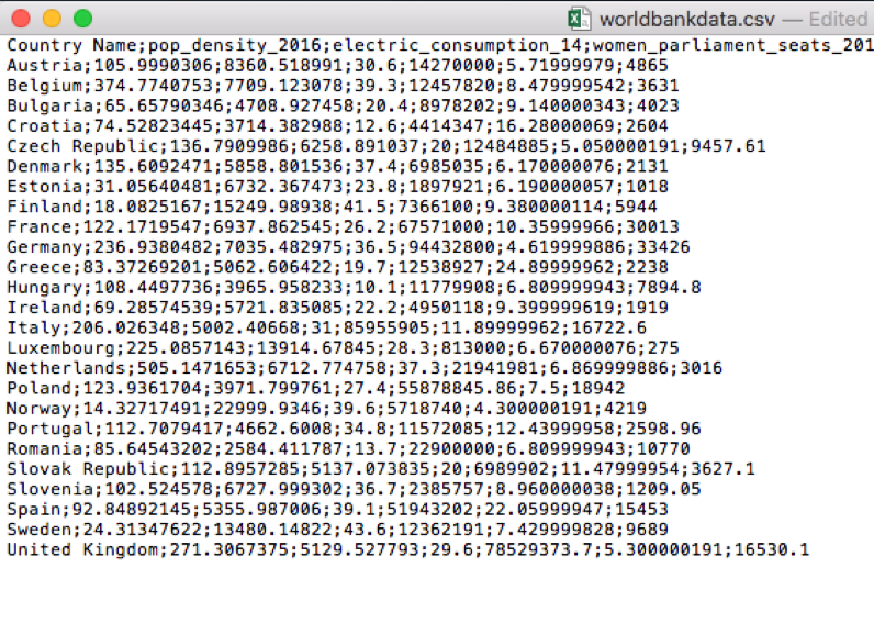
Figure 4.1: Preview of the worldbankdata.csv file
There are 3 things that characterize a csv file:
- the header: the first line containing the names of the variables;
- the field separator (delimiter): the character separating the information (usually the semicolon or the comma is used);
- the decimal separator: the character used for real number decimal points (it can be the full stop or the comma).
In the preview of the csv file reported in Figure 4.1
- the header is given by the following set of strings: Country;pop_density;electric_con;women_seats;mobile;unempl;rail_lines;
- “;” is the field separator;
- “.” is the decimal separator.
All this information are required when importing the data in R by using the read.table (or read.csv) function, whose main arguments are reported here below (see ?read.table):
file: the name of the file which the data are to be read from; this can also including the specification of the folder path (use quotes to specify it);header: a logical value (TorF) indicating whether the file contains the names of the variables as its first line;sep: the field separator character (use quotes to specify it);dec: the character used in the file for decimal points (use quotes to specify it).
Before proceeding with the data import it is good practice to check and then set the working directory. To check which is the current directory we use the function getwd which does not require any input:
## [1] "/Users/michelacameletti/Dropbox/UniBg/Didattica/Economia/2020-2021/CFDS_2021/RCodingforDataScience"To set instead another working directory, where the file worldbankdata.csv is located, we use the setwd function which requires the specification of the path of the folder, as for example in the following case which is referred to my computer (obviously, your path will be different):
To set the working directory, it can be easier to use the RStudio Menu, following Session –> Set Working Directory –> Choose Directory. You choose the directory you want to set as working directory and then click on Open.
The following code is used to import the data available in the worldbankdata.csv file. The output is an object named data:
data = read.csv("worldbankdata.csv",
                 header=T,
                 sep=";", # field separator
                 dec=".") # this can be omitted, it's the default spec.
An alternative for importing data is the user-friendly feature provided by RStudio: read here for more information. The data import feature can be accessed from the environment (top-right) panel (see Figure 4.2). Then all the necessary information can be specified in the following Import Dataset window.
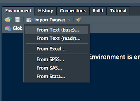
Figure 4.2: The Import Dataset feature of RStudio
After clicking on Import an object named data will be created (essentially this RStudio feature makes use of the read.csv function).
The data is an object of class data.frame:
## [1] "data.frame"Data frames are matrix of data where you can find subjects (in this case Countries) in the rows and variables in the column (in this case you have the following variables: pop_density, electric_con, etc.). A data frame is more general than a matrix, in that different columns be of different type (numeric, character, factor, etc.) but of the same length.
By using str we get information about the type of variables included in the data frame:
## 'data.frame':	25 obs. of  7 variables:
##  $ Country     : chr  "Austria" "Belgium" "Bulgaria" "Croatia" ...
##  $ pop_density : num  106 374.8 65.7 74.5 136.8 ...
##  $ electric_con: num  8361 7709 4709 3714 6259 ...
##  $ women_seats : num  30.6 39.3 20.4 12.6 20 37.4 23.8 41.5 26.2 36.5 ...
##  $ mobile      : num  14270000 12457820 8978202 4414347 12484885 ...
##  $ unempl      : num  5.72 8.48 9.14 16.28 5.05 ...
##  $ rail_lines  : num  4865 3631 4023 2604 9458 ...
In this case the variable Country is interpreted as a qualitative variable (chr stands for characters, a vector of strings) while the other variables (all the prices) are in the form of numerical variables (num).
It is possible to get a preview of the top or bottom part of the data frame by using head or tail:
##          Country pop_density electric_con women_seats   mobile unempl
## 1        Austria   105.99903     8360.519        30.6 14270000   5.72
## 2        Belgium   374.77408     7709.123        39.3 12457820   8.48
## 3       Bulgaria    65.65790     4708.927        20.4  8978202   9.14
## 4        Croatia    74.52823     3714.383        12.6  4414347  16.28
## 5 Czech Republic   136.79100     6258.891        20.0 12484885   5.05
## 6        Denmark   135.60925     5858.802        37.4  6985035   6.17
##   rail_lines
## 1    4865.00
## 2    3631.00
## 3    4023.00
## 4    2604.00
## 5    9457.61
## 6 2131.00## Country pop_density electric_con women_seats mobile unempl
## 20 Romania 85.64543 2584.412 13.7 22900000 6.81
## 21 Slovak Republic 112.89573 5137.074 20.0 6989902 11.48
## 22 Slovenia 102.52458 6727.999 36.7 2385757 8.96
## 23 Spain 92.84892 5355.987 39.1 51943202 22.06
## 24 Sweden 24.31348 13480.148 43.6 12362191 7.43
## 25 United Kingdom 271.30674 5129.528 29.6 78529374 5.30
## rail_lines
## 20 10770.00
## 21 3627.10
## 22 1209.05
## 23 15453.00
## 24 9689.00
## 25 16530.10Use the following alternative function if you want to get information about the dimensions of the data frame:
## [1] 25## [1] 7## [1] 25 74.2 Data selection from a data frame
To select data it is possible to use squared parentheses as seen in Lab 1 for vectors, but in this case two indexes (one for the row and one for the column) will have to be specified. For example the code
## [1] "Croatia"is used to retrieve the element in the 4-th row and 1-st column, corresponding to the name of the 4-th country (Croatia).
If more elements together are requested, a vector of indexes can be used:
## [1] 30.6 39.3 20.4## [1] 30.6 39.3 20.4To select an entire row (i.e. all the information for a given country) you have to specify only the row index:
##   Country pop_density electric_con women_seats  mobile unempl rail_lines
## 4 Croatia    74.52823     3714.383        12.6 4414347  16.28       2604
Similarly, if you are interested in a particular column (i.e. all the values for a given variables), specify only the column index
##  [1] 30.6 39.3 20.4 12.6 20.0 37.4 23.8 41.5 26.2 36.5 19.7 10.1 22.2 31.0 28.3
## [16] 37.3 27.4 39.6 34.8 13.7 20.0 36.7 39.1 43.6 29.6
or alternatively perform the selection by using the $ followed by the column name:
##  [1] 30.6 39.3 20.4 12.6 20.0 37.4 23.8 41.5 26.2 36.5 19.7 10.1 22.2 31.0 28.3
## [16] 37.3 27.4 39.6 34.8 13.7 20.0 36.7 39.1 43.6 29.64.3 Quick exploratory data analysis
Given a vector of data the function summary returns the main summary statistics:
##    Min. 1st Qu.  Median    Mean 3rd Qu.    Max.
##   10.10   20.40   29.60   28.86   37.30   43.60
Variability information are missing. They can be obtained by using the var and sd functions:
## [1] 93.82423## [1] 9.6862914.4 Variable transformation
Let’s assume that we want to transform the quantitative continuous variable women_seats into a qualitative variable taking only two categories:
- Low if women_seats is lower than its first quartile
- High if women_seats is equal to or bigger than its first quartile
First of all note that the first quartile can be computed by using the function quantile as follows:
##  25%
## 20.4
Variable transformation can be performed by using the ifelse function (see also ?ifelse). This function performs a test and then set the two different categories according to the result of the test:
ifelse(data$women_seats < quantile(data$women_seats,0.25),
       "Low", #if the test is TRUE
       "High") #otherwise
## [1] "High" "High" "High" "Low" "Low" "High" "High" "High" "High" "High"
## [11] "Low" "Low" "High" "High" "High" "High" "High" "High" "High" "Low"
## [21] "Low" "High" "High" "High" "High"We want to save the vector given as output in the dataframe. To do this, we proceed by using the $ and specifying directly the new column name (say women_cat):
data$women_cat = ifelse(data$women_seats < quantile(data$women_seats,0.25),
                        "Low", "High")
head(data)
## Country pop_density electric_con women_seats mobile unempl
## 1 Austria 105.99903 8360.519 30.6 14270000 5.72
## 2 Belgium 374.77408 7709.123 39.3 12457820 8.48
## 3 Bulgaria 65.65790 4708.927 20.4 8978202 9.14
## 4 Croatia 74.52823 3714.383 12.6 4414347 16.28
## 5 Czech Republic 136.79100 6258.891 20.0 12484885 5.05
## 6 Denmark 135.60925 5858.802 37.4 6985035 6.17
## rail_lines women_cat
## 1 4865.00 High
## 2 3631.00 High
## 3 4023.00 High
## 4 2604.00 Low
## 5 9457.61 Low
## 6 2131.00 High## 'data.frame': 25 obs. of 8 variables:
## $ Country : chr "Austria" "Belgium" "Bulgaria" "Croatia" ...
## $ pop_density : num 106 374.8 65.7 74.5 136.8 ...
## $ electric_con: num 8361 7709 4709 3714 6259 ...
## $ women_seats : num 30.6 39.3 20.4 12.6 20 37.4 23.8 41.5 26.2 36.5 ...
## $ mobile : num 14270000 12457820 8978202 4414347 12484885 ...
## $ unempl : num 5.72 8.48 9.14 16.28 5.05 ...
## $ rail_lines : num 4865 3631 4023 2604 9458 ...
## $ women_cat : chr "High" "High" "High" "Low" ...We note that there is a new column in the data frame of type chr. If we try to apply the summary function to this new variable we get something meaningless:
##    Length     Class      Mode
##        25 character character
In R it is better, also in terms of statistical analys, the qualitative variables into factor object. A factor object is used to define categorical (nominal or ordered) variables. It can be viewed as an integer vector where each integer value has a corresponding label. It’s more convenient than a vector of characters (chr) as each unique character value is stored only once, and the data itself is stored as a vector of integers. We create the factor object by using the factor function (see also ?factor) and we save it in a new column of the data frame named women_fact:
##          Country pop_density electric_con women_seats   mobile unempl
## 1        Austria   105.99903     8360.519        30.6 14270000   5.72
## 2        Belgium   374.77408     7709.123        39.3 12457820   8.48
## 3       Bulgaria    65.65790     4708.927        20.4  8978202   9.14
## 4        Croatia    74.52823     3714.383        12.6  4414347  16.28
## 5 Czech Republic   136.79100     6258.891        20.0 12484885   5.05
## 6        Denmark   135.60925     5858.802        37.4  6985035   6.17
##   rail_lines women_cat women_fact
## 1    4865.00      High       High
## 2    3631.00      High       High
## 3    4023.00      High       High
## 4    2604.00       Low        Low
## 5    9457.61       Low        Low
## 6 2131.00 High High## 'data.frame': 25 obs. of 9 variables:
## $ Country : chr "Austria" "Belgium" "Bulgaria" "Croatia" ...
## $ pop_density : num 106 374.8 65.7 74.5 136.8 ...
## $ electric_con: num 8361 7709 4709 3714 6259 ...
## $ women_seats : num 30.6 39.3 20.4 12.6 20 37.4 23.8 41.5 26.2 36.5 ...
## $ mobile : num 14270000 12457820 8978202 4414347 12484885 ...
## $ unempl : num 5.72 8.48 9.14 16.28 5.05 ...
## $ rail_lines : num 4865 3631 4023 2604 9458 ...
## $ women_cat : chr "High" "High" "High" "Low" ...
## $ women_fact : Factor w/ 2 levels "High","Low": 1 1 1 2 2 1 1 1 1 1 ...Note that different structure reported by str. Moreover, it is now possible to use the summary function:
## High  Low
##   19    6
that returns the frequency distribution of this categorical variable. Given this, it is also possible to do some conditional plotting by using, for example, a boxplot:
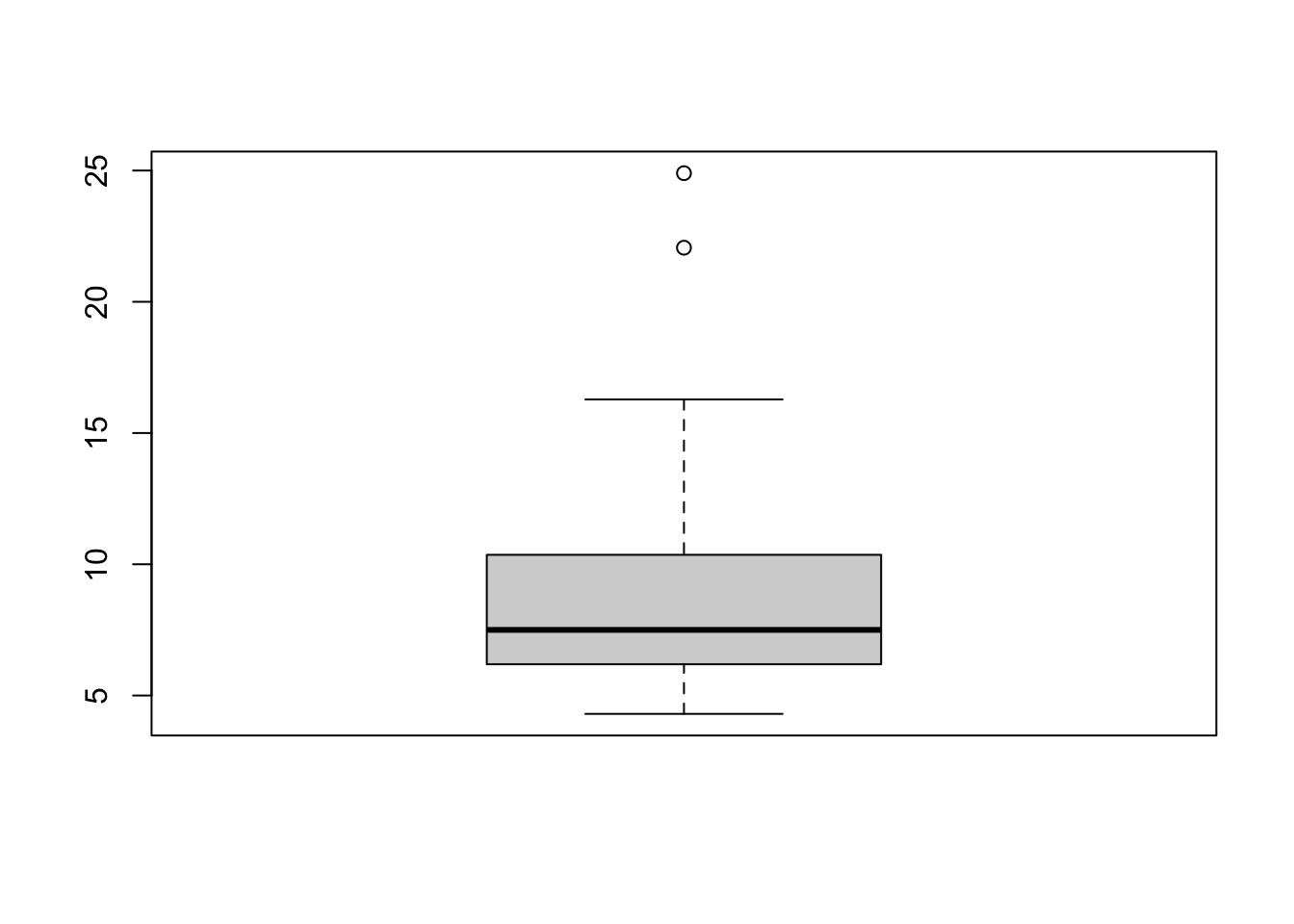
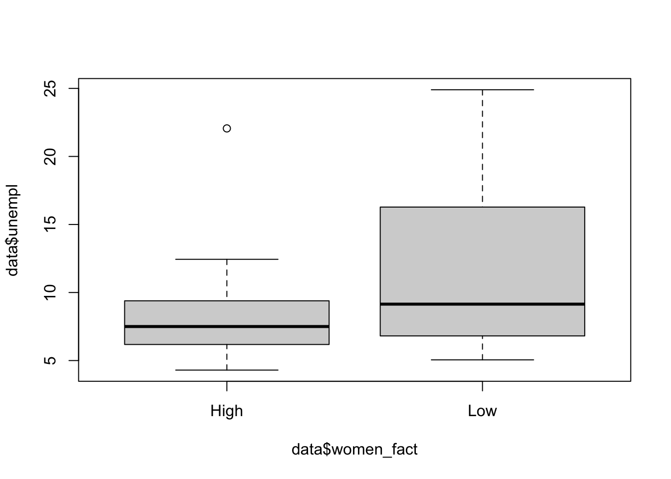 The first is the boxplot representing the marginal distribution of the unemployment rate; the second instead represents the distribution of the unemployment rate conditioning on the two categories of
 women_fact. The ~ should be read as as a function of.
4.5 Apply a function by column
Let’s assume that you want to compute a function, e.g. the mean, for all the quantitative variables in your data frame. You can proceed by writing separate lines of code, one for each variable:
## [1] 137.5793## [1] 7319.844## [1] 28.856## [1] 24684722## [1] 9.3688## [1] 8488.649Alternatively, you can use the apply function for applying the same function (mean) to all (or some) columns of your data frame. This is the requested code:
##  pop_density electric_con  women_seats       mobile       unempl   rail_lines
## 1.375793e+02 7.319844e+03 2.885600e+01 2.468472e+07 9.368800e+00 8.488649e+03
The first input of the function is the selection of quantitative columns, 2 is the specification of the MARGIN argument of the function (see ?apply) and refers to the fact that you want to apply the function by column (set 1 if by row). Finally, mean is the function you are interested in. It is also possible to use another function:
##  pop_density electric_con  women_seats       mobile       unempl   rail_lines
## 5.051472e+02 2.299993e+04 4.360000e+01 9.443280e+07 2.490000e+01 3.342600e+04## pop_density electric_con women_seats mobile unempl rail_lines
## 1.297045e+04 2.059069e+07 9.382423e+01 8.353452e+14 2.597143e+01 7.860576e+07The same selection of columns can be obtained by using
##  pop_density electric_con  women_seats       mobile       unempl   rail_lines
## 1.375793e+02 7.319844e+03 2.885600e+01 2.468472e+07 9.368800e+00 8.488649e+03
where the - can be used to remove some of the columns in the data frame (in this case the columns referring to qualitative variables for which it is not possible to compute the mean).
4.6 Exercises Lecture 2
4.6.1 Exercise 1
The data in the WHI2017.csv file refer to the World Happiness report, 2017 (https://www.kaggle.com/unsdsn/world-happiness/home). The available variables are the following:
Country: Name of the countryHappiness.Rank: Rank of the country based on the Happiness Score.Happiness.Score: A metric measured in 2017 by asking the sampled people the question: “How would you rate your happiness on a scale of 0 to 10 where 10 is the happiest?”.Economy.GDP.per.Capita: The extent to which GDP contributes to the calculation of the Happiness Score.Family: The extent to which Family contributes to the calculation of the Happiness Score.Health.Life.Expectancy: The extent to which Life expectancy contributed to the calculation of the Happiness Score.Freedom: The extent to which Freedom contributed to the calculation of the Happiness Score.Generosity: The extent to which Generosity contributed to the calculation of the Happiness Score.Trust.Gov.Corr: The extent to which Perception of Government Corruption contributes to Happiness Score.Dystopia.Residual: The extent to which Dystopia Residual contributed to the calculation of the Happiness Score.
The columns following the happiness score estimate the extent to which each of six factors – economic production, social support, life expectancy, freedom, absence of corruption, and generosity – contribute to making life evaluations higher in each country than they are in Dystopia, a hypothetical country that has values equal to the world’s lowest national averages for each of the six factors.
Set your working directory and then import the data in
R.For the first two countries (Norway and Denmark) check that the sum of the values in the columns from
Economy.GDP.per.CapitatoDystopia.Residualis equal to the value of theHappines.Scorevariable (apart from rounding).Study the distribution of
Happiness.Scoreby computing some summary statistics. Do you observe something strange given the variable definitions?Find the country associated with the error in the data (see previous point) and remove it from the data. You have to perform a selection by condition as described in Lecture 1.
Plot the distribution of
Happiness.Scoreby using an histogram. Add to the plot three vertical lines denoting the quartiles; you can do this by using theablinefunction (see?abline). Moreover, add to the plot a vertical line for the Italian score.Which are the countries with an Happiness score lower than the first quartile? And which are over the third quartile?
Plot the distribution of
Happiness.Scoreby using a boxplot. Do you observe any outliers?Classify the
Happiness.Scoreinto a new variable namedHappiness.Score.2which takes three values: -1 ifHappiness.Score<= first quartile, 0 ifHappiness.Scoreis between the first and third quartile and +1 ifHappiness.Scoreis >= the third quartile. Compute the absolute/relative frequency table forHappiness.Score.2and plot it. Suggestion: you have to nestifelseinside anotherifelsefunction.Transform
Happiness.Score.2into a categorical variable (factor) with the following labels: low, medium, high (set the labels by using thelabelsargument of thefactorfunction). Compute the frequency distribution withsummary.Create a new variable
GDP.propwich is defined as the proportion of the Happiness score given byEconomy.GDP.per.Capita. Compute some summary statistics.Plot the distribution of
GDP.propgiven (conditional on) the levels ofHappiness.Score.2. What can you conclude?Consider Italy. Which are the most and less important factors (among economic production, social support, life expectancy, freedom, absence of corruption, and generosity) affecting happiness? Do you observe the same for the country with the highest happiness score?