Chapter 3 R Lab 2 - 29/03/2023
In this lecture we will learn how to implement the logistic regression model and the linear discriminant analysis (LDA).
The following packages are required: tidyverse,tidymodels and discrim.
library(tidymodels)
library(tidyverse)
#install.packages('discrim') # needed for LDA
library(discrim)
##
## Attaching package: 'discrim'## The following object is masked from 'package:dials':
##
## smoothness3.1 Satisfaction data
The data we use for this lab are from the Kaggle platform link. You can download the dataset from Moodle (the file is satisf.csv).
The objective of the analysis is to predict whether or not a customer is overall satisfied with the company service, based on other quality measurements.The datasets consists of several predictor variables:
outcome: Customer’s overall satisfaction about the airline (0 = Neutral or dissatisfied, 1 = Satisfied)age: Age of passenger (years)dist: Flight distance of the evaluated journey (not indicated :-( )dep_delay: Delay when departure (minutes)arr_delay: Delay delayed at the arrival (minutes)
The response variable is named outcome and is a binary variable: 0 means that the customer was not satisfied about the overall company service, while 1 means he/she was pleased by the experience.
We import the data
satisf <- read.csv("./files/satisf.csv")
glimpse(satisf)
## Rows: 129,487
## Columns: 5
## $ outcome <int> 1, 1, 0, 1, 1, 1, 1, 1, 1, 1, 1, 0, 1, 1,…
## $ age <int> 52, 36, 20, 44, 49, 16, 77, 43, 47, 46, 4…
## $ dist <int> 160, 2863, 192, 3377, 1182, 311, 3987, 25…
## $ dep_delay <int> 50, 0, 0, 0, 0, 0, 0, 77, 1, 28, 29, 18, …
## $ arr_delay <int> 44, 0, 0, 6, 20, 0, 0, 65, 0, 14, 19, 7, …We transform the outcome 0/1 integer variable into a factor with categories “Neutral or dissatisfied” and “Satisfied”:
satisf$outcome= factor(satisf$outcome)
levels(satisf$outcome) = c("Neutral-Dissatisfied","Satisfied")
table(satisf$outcome)
##
## Neutral-Dissatisfied Satisfied
## 73225 56262Some exploratory analysis can be done to study the distribution of the regressors conditionally on the satisfaction condition. We consider here, as an example, Age or Distance:
satisf %>%
  ggplot() +
  geom_boxplot(aes(age,fill=outcome))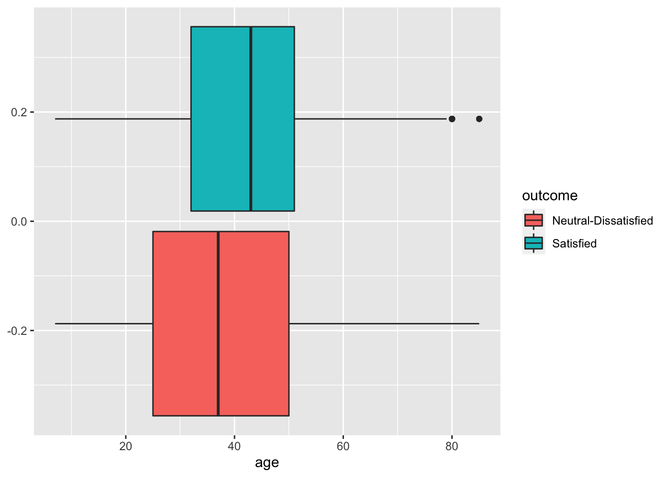
# It seems that the most satisfied customers are also the older ones

satisf %>%
  ggplot() +
  geom_density(aes(dist,fill=outcome),alpha=0.3)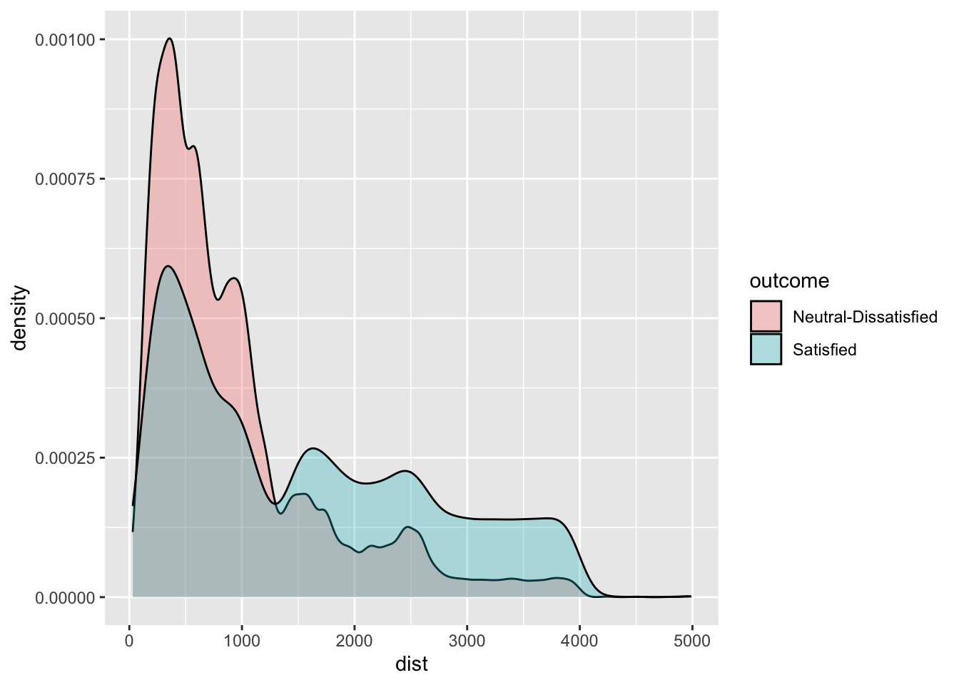
# Satisfaction seems to be related also to travel distance. Passenger travelling on longer flights are the one
# that face less dissatisfaction/neutrality.
3.2 Definition of a function for computing performance indexes
For assessing the performance of a classifier we compare predicted categories with observed categories. This can be done by using the confusion matrix which is a 2x2 matrix reporting the joint distribution (with absolute frequencies) of predicted (by row) and observed (by column) categories.
| No (obs.) | Yes (obs.) | |||
|---|---|---|---|---|
| No (pred.) | TN | FN | ||
| Yes (pred.) | FP | TP | ||
| Total | N | P |
We consider in particular the following performance indexes:
- sensitivity (true positive rate): TP/P
- specificity (true negative rate): TN/N
- accuracy (rate of correctly classified observations): (TN+TP)/(N+P)
We define a function named perf_indexes which computes the above defined indexes. The function has only one argument which is a confusion 2x2 matrix named cm. It returns a vector with the 3 indexes.
perf_indexes = function(cm){
  sensitivity = cm[2,2] / (cm[1,2] + cm[2,2])
  specificity = cm[1,1] / (cm[1,1] + cm[2,1])
  accuracy = sum(diag(cm)) / sum(cm)
  return(c(sens=sensitivity,spec=specificity,acc=accuracy))
}
3.3 A new method for creating the training and testing set
To create the training (80%) and test (20%) dataset we use a new approach different from the one introduced in Section 2.2.1 and Section 2.3.
We first create a vector with the indexes we will use for the training dataset by using the sample function. In this case we must set replace to FALSE, since each index will indicate an observation belonging to just train or test. Recall also to set a seed, in order to be able to replicate your results:
set.seed(11, sample.kind="Rejection")
training_index = sample(1:nrow(satisf),
                         0.8*nrow(satisf),
                         replace=F) # notice that here resample is not allowed!
head(training_index)
## [1] 65570 66457 128113 19004 73612 28886We are now ready to sample from the satisf dataset 80% of the observations (rows) by using the training_index vector, and leave the non-sampled indexes for test. We use the %in% operator to find out which elements of a vector are present in another vector:
s_train = satisf %>%
  filter(row_number() %in% training_index)
s_test = satisf %>%
  filter(!row_number() %in% training_index)

# check datasets
head(s_train)
## outcome age dist dep_delay arr_delay
## 1 Satisfied 52 160 50 44
## 2 Satisfied 36 2863 0 0
## 3 Neutral-Dissatisfied 20 192 0 0
## 4 Satisfied 44 3377 0 6
## 5 Satisfied 16 311 0 0
## 6 Satisfied 77 3987 0 0head(s_test)## outcome age dist dep_delay arr_delay
## 1 Satisfied 49 1182 0 20
## 2 Neutral-Dissatisfied 33 325 18 7
## 3 Neutral-Dissatisfied 43 1927 0 0
## 4 Satisfied 44 1543 0 0
## 5 Neutral-Dissatisfied 51 235 0 0
## 6 Neutral-Dissatisfied 22 1846 40 68Note that this procedure could be the easiest choice when we don’t have a third dataset (validation).
We are now ready to train our models.
3.4 Logistic regression
For implementing the logistic regression the function logistic_reg() is used. It requires the specification of the engine, and the mode as you can see in the picture taken from https://www.tidymodels.org/find/parsnip/:
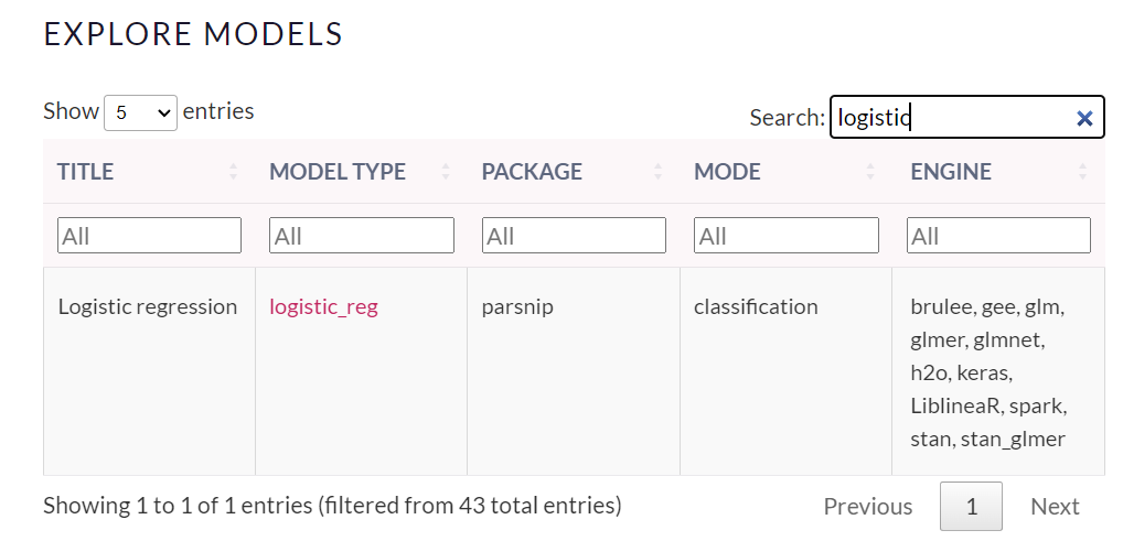
# Create a logistic regression model specification
logreg_spec <- logistic_reg() %>%
  set_engine("glm") %>%
  set_mode("classification")

# Fit the logistic regression model
logreg_fit <- logreg_spec %>%
  fit(outcome ~ ., data = s_train)
# Print the model summary
summary(logreg_fit$fit)
##
## Call:
## stats::glm(formula = outcome ~ ., family = stats::binomial, data = data)
##
## Deviance Residuals:
## Min 1Q Median 3Q Max
## -2.2647 -0.9716 -0.7758 1.1563 2.5771
##
## Coefficients:
## Estimate Std. Error z value Pr(>|z|)
## (Intercept) -1.556e+00 2.037e-02 -76.361 < 2e-16 ***
## age 1.522e-02 4.403e-04 34.572 < 2e-16 ***
## dist 6.214e-04 7.038e-06 88.294 < 2e-16 ***
## dep_delay 3.118e-03 6.908e-04 4.514 6.37e-06 ***
## arr_delay -6.788e-03 6.842e-04 -9.921 < 2e-16 ***
## ---
## Signif. codes:
## 0 '***' 0.001 '**' 0.01 '*' 0.05 '.' 0.1 ' ' 1
##
## (Dispersion parameter for binomial family taken to be 1)
##
## Null deviance: 141820 on 103588 degrees of freedom
## Residual deviance: 130815 on 103584 degrees of freedom
## AIC: 130825
##
## Number of Fisher Scoring iterations: 4Note that the notation outcome ~. means that all the covariates but outcome are included as regressors (this avoids to write the formula in the standard way: outcome ~ age+dist+...).
The summary contains the parameter estimates and the corresponding p-values of the test checking \(H_0:\beta =0\) vs \(H_1: \beta\neq 0\). Consider for example the parameter of the Age variable which is positive (i.e. higher possibility of being satisfied) and equal to 0.0152229: this means that for a one-unit increase in age, the log-odds increases by 0.0152229. For a simpler interpretation, in the odds scale, we can take the exponential transformation of the parameter:
# odds ratio
exp(logreg_fit$fit$coefficients[2])
## age
## 1.015339# odds interpretation
(exp(coef(logreg_fit$fit)[2]) -1)*100## age
## 1.533937This means that for a one-unit increase in the customer’s age, we expect a 1.53 percent increase in the satisfaction odds. Remember that the odds is strictly connected to the satisfaction probability as it is defined as \(p/(1-p)\)).
We are now interested in computing predictions for the test observations given the estimated logistic model. They can be obtained by using the predict function. It is important to specify that we are interested in the prediction on the outcome scale (otherwise we will get the predictions on the logit scale):
logreg_pred = logreg_fit %>% predict(new_data = s_test, type="prob")
head(logreg_pred)
## # A tibble: 6 × 2
## `.pred_Neutral-Dissatisfied` .pred_Satisfied
## <dbl> <dbl>
## 1 0.553 0.447
## 2 0.699 0.301
## 3 0.426 0.574
## 4 0.482 0.518
## 5 0.653 0.347
## 6 0.601 0.399The tibble logreg_pred contains the conditional probability of being ‘satisfied’ and ‘Neutral-Dissatisfied’ given the covariate vector. For example for the first test observation the satisfaction probability is equal to logreg_pred$.pred_Satisfied[1]. In order to have a categorical prediction it is necessary to fix a threshold for the probability (default is 0.5) and transform correspondingly the probabilities:
logreg_pred$pred = ifelse(logreg_pred$.pred_Satisfied > 0.5, "Satisfied", "Neutral-Dissatisfied")
logreg_pred$pred = factor(logreg_pred$pred)
As expected, the predicted category for the first observation is “Neutral - Dissatisfied”.
We are now ready to compute the confusion matrix
#with table function
table(logreg_pred$pred, s_test$outcome)
##
## Neutral-Dissatisfied Satisfied
## Neutral-Dissatisfied 12117 6259
## Satisfied 2524 4998#you can also calculate with conf_mat() function
logreg_pred = logreg_pred %>%
mutate(actual = s_test$outcome)
confusion_mat = logreg_pred %>%
conf_mat(truth = actual, estimate = pred)
confusion_mat## Truth
## Prediction Neutral-Dissatisfied Satisfied
## Neutral-Dissatisfied 12117 6259
## Satisfied 2524 4998and the performance index by using the function we defined in Section 3.2
perf_indexes(table(logreg_pred$pred, s_test$outcome))## sens spec acc
## 0.4439904 0.8276074 0.6608618What happen to our performance indexes if we change prediction threshold?
logreg_pred$pred = ifelse(logreg_pred$.pred_Satisfied > 0.8, "Satisfied", "Neutral-Dissatisfied")
logreg_pred$pred = factor(logreg_pred$pred)
perf_indexes(table(logreg_pred$pred, s_test$outcome))
## sens spec acc
## 0.04557164 0.99112083 0.58012202As you can see, increasing the satisfaction threshold can improve a lot the algorithm specificity (= our algorithm is more able to detect an unsatisfied customer). At the same time, the decreased in the sensitivity and overall accuracy should be considered. In general, the decision of lowering / increasing the decision boundary depends on the context we are applying our knowledge. Think about COVID. Should be “better” to have a diagnostic test with more false positive (= lower specificity) or false negative (= lower sensitivity)?
3.5 Linear discriminant analysis
To run LDA we use the discrim_linear() function of the parsnip package. See in the following picture the function and the different engines we can use (taken from https://www.tidymodels.org/find/parsnip/):
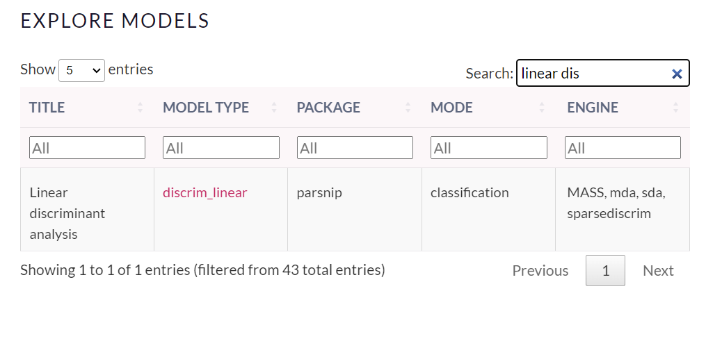
Similarly to logistic regression we have to create the specifications, engine and the mode:
# Create an LDA model specification
lda_spec <- discrim_linear() %>%
  set_engine("MASS") %>%
  set_mode("classification")

# Fit the LDA model
lda_fit <- lda_spec %>%
  fit(outcome ~ ., data = s_train)
# Print the LDA model
lda_fit
## parsnip model object
##
## Call:
## lda(outcome ~ ., data = data)
##
## Prior probabilities of groups:
## Neutral-Dissatisfied Satisfied
## 0.5655427 0.4344573
##
## Group means:
## age dist dep_delay arr_delay
## Neutral-Dissatisfied 37.66313 928.5023 16.29445 17.02332
## Satisfied 41.73423 1526.8704 12.22791 12.36638
##
## Coefficients of linear discriminants:
## LD1
## age 0.0226054119
## dist 0.0009458021
## dep_delay 0.0045190445
## arr_delay -0.0093103673The output reports the prior probabilities for the two categories and the conditional means of all the covariates. Recall that the prior probability is the probability that a randomly chosen observation comes from the \(k^{th}\) class.
We go straight to the calculation of the predictions. In this case it is possible to specify which is the output of the predict function (the probabilities of the response categories):
lda_pred = lda_fit %>% predict(new_data = s_test, type = 'prob')
head(lda_pred)
## # A tibble: 6 × 2
## `.pred_Neutral-Dissatisfied` .pred_Satisfied
## <dbl> <dbl>
## 1 0.557 0.443
## 2 0.709 0.291
## 3 0.428 0.572
## 4 0.486 0.514
## 5 0.664 0.336
## 6 0.598 0.402lda_pred = lda_pred %>%
bind_cols(lda_fit %>% predict(new_data = s_test, type = 'class'))Note that the tibble lda_pred is a tibble having 3 variables including posterior probabilities of each class and the vector of predicted categories:
head(lda_pred)## # A tibble: 6 × 3
## `.pred_Neutral-Dissatisfied` .pred_Satisfied .pred_class
## <dbl> <dbl> <fct>
## 1 0.557 0.443 Neutral-Dissa…
## 2 0.709 0.291 Neutral-Dissa…
## 3 0.428 0.572 Satisfied
## 4 0.486 0.514 Satisfied
## 5 0.664 0.336 Neutral-Dissa…
## 6 0.598 0.402 Neutral-Dissa…To compute the confusion matrix we will use the vector lda_pred$.pred_class:
table(lda_pred$.pred_class, s_test$outcome)##
## Neutral-Dissatisfied Satisfied
## Neutral-Dissatisfied 12179 6306
## Satisfied 2462 4951perf_indexes(table(lda_pred$.pred_class, s_test$outcome))## sens spec acc
## 0.4398152 0.8318421 0.6614410As before, we can choose a different threshold for our decision. In this case, the used functions do not allow to change directly the threshold. So, we need to use the same methodology applied to logistic regression classification method to generate new class. Recall that LDA assigns the observation to the most likely class (= class with highest posterior probability). So, there is an implicit probability threshold with two classes (\(0.5\)). Check it by yourself here above:
lda_pred$pred = ifelse(lda_pred$.pred_Satisfied > 0.5, "Satisfied", "Neutral-Dissatisfied")
# same results than previous LDA
table(lda_pred$pred, s_test$outcome)
##
## Neutral-Dissatisfied Satisfied
## Neutral-Dissatisfied 12179 6306
## Satisfied 2462 4951# same results than previous LDA
perf_indexes(table(lda_pred$pred, s_test$outcome))## sens spec acc
## 0.4398152 0.8318421 0.6614410We can now set an higher probability threshold, with the aim of being able to better select the “real” satisfied customers. The probability threshold will be set on the “Satisfied” class at \(0.8\) :
lda_pred$pred = ifelse(lda_pred$.pred_Satisfied > 0.8, "Satisfied", "Neutral-Dissatisfied")

table(lda_pred$pred, s_test$outcome) #objects are changed w.r.t. before
##
## Neutral-Dissatisfied Satisfied
## Neutral-Dissatisfied 14499 10673
## Satisfied 142 584perf_indexes(table(lda_pred$pred, s_test$outcome)) #objects are changed w.r.t. before## sens spec acc
## 0.05187883 0.99030121 0.58240019We reduced a lot the false positive observation (from \(2462\) to \(142\)). We were able to correctly detect more real unsatisfied customers (from \(12179\) to \(14499\)), increasing the specificity of our algorithm. However, we dramatically predict with a wrong class lots of truly satisfied customers (\(6306\) to \(10673\)), being able to predict very few true “positive” (Satisfied) travelers (\(584\)).
3.6 Classifiers comparison in terms of performance indexes
By comparing the 2 classifiers with respect to accuracy, sensitivity and specificity
perf_indexes(table(logreg_pred$pred, s_test$outcome))## sens spec acc
## 0.04557164 0.99112083 0.58012202perf_indexes(table(lda_pred$pred, s_test$outcome))## sens spec acc
## 0.05187883 0.99030121 0.58240019We see that the logistic regression and LDA perform very similarly. In particular, Logistic regression has the highest specificity but the lowest sensitivity. In terms of accuracy LDA has the best performance.
3.7 Exercises Lab 2
3.7.1 Exercise 1
The data contained in the files titanic_tr.csv (for training) and titanic_te.csv (and testing) are about the Titanic disaster (the files are available in the e-learning). In particular the following variables are available:
pclass: ticket class (1 = 1st, 2 = 2nd, 3 = 3rd)survived: survival (0 = No, 1 = Yes)nameof the passengersexagein years
sibsp: number of siblings / spouses aboard the Titanic
parchnumber of parents / children aboard the Titanic
ticket: ticket number
fare: passenger fare
cabin: cabin number
embarked: port of Embarkation (C = Cherbourg, Q = Queenstown, S = Southampton)
Import the data in R and explore them. Note that the response variable is survived which is classified as a int 0/1 variable in the dataframe. Transform it in a factor type object using the factor function with categories “No” and “Yes”.
Convert
pclass(ticket class) to factor (1 = “1st”, 2 = “2nd”, 3 = “3rd”) for both the training and test data set. Plotsurvivedas a function ofpclass. In which class do you observe the highest proportion of survivors?Check how many missing values we have in the variables
ageandfareseparately for training and test data.
- Separately for the training and test data, substitute the missing values with the average of
ageandfare. Note that for computing the mean when you have missing values you have to runmean(...,na.rm=T). After this, check that you don’t have any other missing values.
Consider the training data and
survivedas response variable. Compute the percentage of survived people. Moreover, represent graphically the relationship betweenageandsurvived. Comment the plot.Consider the training data set, estimate a logistic model for
survivedconsideringageas the only predictor (mod1). Provide the model summary.
Comment the
agecoefficient.Compute manually (without using
predict) by means of the formula of the logistic function the probability of surviving for a person of 50 years old. Remember that estimated coefficients can be retrieved bymod1$coefficients. Repeat the same for a person of 20 years old. Finally compute the odds and the odds-ratio.Compute the probability of surviving for all the people in the test data set (use
predict).Plot the estimated probabilities as a function of age (impose that the probability axis is between 0 and 1). Use for each point a color corresponding to the
survivedoutcome. Moreover, include in the plot an horizontal line corresponding to the probability threshold (0.5) and the corresponding age threshold (age boundary between categories). Comment the plot.Compute the confusion matrix for
mod1. Moreover, compute the test classification error rate.
- Consider the training data set, estimate a logistic model for
survivedconsideringpclassas predictor (mod2). Note thatpclassis a categorical variable with 3 categories and will be included in the model as a dummy variable with 3-1 categories (one category is the baseline). Provide the model summary and comment the coefficients. The following functioncontrastshelps you in understanding which is the baseline category:
contrasts(tr$pclass)
# on the rows you have the categories
# on the column the 2 dummy variables that will be included in the model (for the 2nd and 3rd category)
#the baseline is the category 1st
#in the model 2 coefficients will be estimated for category 2nd and 3rd
For more information about the management of dummy variables in R please read this short note available here. It refers to a linear regression model but it generalizes to any model.
Compute (manually or by using
predict) the probability of surviving for a person with a 1st class ticket. Repeat also for the other 2 classes. Compare the three predicted probabilities with the corresponding surviving proportion computed for each class.Estimate the probability of surviving (and the corresponding categories) for all the observations in the test data set (using
predict). Then compute the test overall classification error rate and compare it with the one obtained formod1.
For the training observations represent graphically
fare(amount paid for the ticket) as a function ofpclass. Moreover, compute the average and medianfareamount separately for each class.Consider the training data set, estimate a logistic model for
survivedconsideringageandfareas predictors (mod3). Provide the model summary.
Comment the coefficient of
fare.Using
mod3compute the predicted probability of surviving for all the test observations and the corresponding categories.Plot
fare(y-axis) as a function ofageusing the predicted categories to color the points. Moreover, include in the plot the linear boundary (it’s the solution of \(\beta_0+\beta_1 X_1+\beta_2X_2=0\)) which separates the two groups. HINT: derive it considering \(X_2 = Y\) and \(\beta_1=X\).Given the previous plot, what’s the prediction for a 40 years old individual who paid 200 dollars ?
Compute the test error rate for
mod3and compare it with the other models.
- Consider the training data set, estimate a logistic model for
survivedconsideringage,fareandpclassas predictors (mod4). Provide the model summary. Comparemod4with the others by using the test classification error. Which is the best model?
3.7.2 Exercise 2
We will use some simulated data available from the mlbench library (don’t forget to install it) with \(p=2\) regressors and a binary response variable. Use the following code to generate the data and create the data frame.
library(mlbench)

?mlbench.circle
set.seed(3333,sample.kind="Rejection")
data = mlbench.circle(1000) #simulate 1000 data
datadf = data.frame(data$x,
                    Y=factor(data$classes,labels=c("No","Yes")))
head(datadf)
## X1 X2 Y
## 1 0.4705415 -0.52006500 No
## 2 -0.1253492 0.20921556 No
## 3 -0.4381452 0.52445868 No
## 4 0.5877131 -0.86523067 Yes
## 5 0.1631693 -0.01084204 No
## 6 -0.6190528 -0.98775598 YesPlot the data (use the response variable to color the points).
Split the dataset in two parts: 80% of the observations are used for training and 20% for testing. The split is random (use as seed for random number generation the number 456).
Estimate a logistic regression model using
X1andX2as regressors. Provide the model summary.Comment the model coefficients.
Plot the training data and add to the plot the linear decision boundary (see the slides for the formula) defined by the logistic model. Do you think that the model is working well?
Compute the predictions using the test observations. Provide the confusion matrix (use 0.5 as probability threshold) and the overall classification error rate.
Define a function named
classification_perfwhich computes the overall classification error rate, the sensitivity and the specificity for a 2x2 confusion matrix which has in the rows the predicted categories and in the columns the observed categories.Use the
classification_perffunction for the logistic regression model output. Comment about the performance of the logistic regression model.Consider now a very simple classifier (null classifier) which uses as prediction for all the test observations the majority class observed in the training dataset (regardless of the values of the predictors). Compute the overall error rate for the null classifier. Does it perform better than the logistic regression model?
Use linear discriminant analysis to classify your data. Compute the predictions using the test observations and provide the confusion matrix together with performance indexes. Comment the results.
- [Advanced and optional] Using a grid of values for
X1andX2together with theouterfunction, plot the decision boundary together with the training data. Add to the plot also the boundary estimated with the logistic model.
- [Advanced and optional] Using a grid of values for
Compare the three previous classifier (LR, null classifier, LDA) using the confusion matrix (with the
classification_perfformula) and the error rate. Are you able to compute the performance indexes with the null classifier? Which of the proposed model seems to perform better?
3.7.3 Exercise 3
We will use some simulated data available from the mlbench library with \(p=2\) regressors and a response variable with 4 categories. Use the following code to generate the data.
library(mlbench)

?mlbench.smiley
set.seed(3333,sample.kind="Rejection")
data = mlbench.smiley(1000) #simulate 1000 data
datadf = data.frame(data$x, factor(data$classes))
head(datadf)
## x4 V2 factor.data.classes.
## 1 -0.7371167 0.9282289 1
## 2 -0.8580089 1.0668791 1
## 3 -0.7794051 1.0191270 1
## 4 -0.9232296 0.9328375 1
## 5 -0.7723922 0.9318714 1
## 6 -0.9142181 0.8255049 1colnames(datadf) = c("x1", "x2", "y")
head(datadf)## x1 x2 y
## 1 -0.7371167 0.9282289 1
## 2 -0.8580089 1.0668791 1
## 3 -0.7794051 1.0191270 1
## 4 -0.9232296 0.9328375 1
## 5 -0.7723922 0.9318714 1
## 6 -0.9142181 0.8255049 1table(datadf$y)##
## 1 2 3 4
## 167 167 250 416Plot the data (use the response variable to color the points).
Split the dataset in two parts: 70% of the observations are used for training and 20% for testing. The split is random (use as seed for random number generation the number 456).
Consider linear discriminant analysis for your data. Analyse your results computing the test error rate.
Use the KNN method to classify your data. Choose the best value of \(k\) among a sequence of values between 1 and 100 (with step equal to 5). To tune the hyperparameter \(k\) split the training dataset into two sets: one for training (70%) and one for validation (30%). Use a seed equal to 4.
Which model (between lda and knn) do you prefer? Explain why.