Chapter 6 R Lab 5 - 10/05/2023
In this lecture we will learn how to implement gradient boosting (regression) and adaboost.M1 (binary classification). We will then compare the performances of gradient boosting to other regression methods.
The following packages are required: MASS, fastAdaboost,tidymodels, gbm and tidyverse.
library(MASS) # for our dataset##
## Attaching package: 'MASS'## The following object is masked from 'package:dplyr':
##
## selectlibrary(tidymodels)
library(tidyverse) # data management
library(gbm) #for gradient boosting## Loaded gbm 2.1.8library(fastAdaboost)# for adaboostWe first load the library MASS which contains the dataset Boston (Housing Values in Suburbs of Boston, see ?Boston for the description of the variables). Our response variable would be medv, and the others will be used as regressors.
glimpse(Boston)## Rows: 506
## Columns: 14
## $ crim <dbl> 0.00632, 0.02731, 0.02729, 0.03237, 0.06905…
## $ zn <dbl> 18.0, 0.0, 0.0, 0.0, 0.0, 0.0, 12.5, 12.5, …
## $ indus <dbl> 2.31, 7.07, 7.07, 2.18, 2.18, 2.18, 7.87, 7…
## $ chas <int> 0, 0, 0, 0, 0, 0, 0, 0, 0, 0, 0, 0, 0, 0, 0…
## $ nox <dbl> 0.538, 0.469, 0.469, 0.458, 0.458, 0.458, 0…
## $ rm <dbl> 6.575, 6.421, 7.185, 6.998, 7.147, 6.430, 6…
## $ age <dbl> 65.2, 78.9, 61.1, 45.8, 54.2, 58.7, 66.6, 9…
## $ dis <dbl> 4.0900, 4.9671, 4.9671, 6.0622, 6.0622, 6.0…
## $ rad <int> 1, 2, 2, 3, 3, 3, 5, 5, 5, 5, 5, 5, 5, 4, 4…
## $ tax <dbl> 296, 242, 242, 222, 222, 222, 311, 311, 311…
## $ ptratio <dbl> 15.3, 17.8, 17.8, 18.7, 18.7, 18.7, 15.2, 1…
## $ black <dbl> 396.90, 396.90, 392.83, 394.63, 396.90, 394…
## $ lstat <dbl> 4.98, 9.14, 4.03, 2.94, 5.33, 5.21, 12.43, …
## $ medv <dbl> 24.0, 21.6, 34.7, 33.4, 36.2, 28.7, 22.9, 2…Since we don’t have a classification variable in our dataset, we create it dividing the response variable into two classes: “high”, with values of medv above or equal to the median value of medv, and low for values below this threshold.
b.dt <- Boston # save in a new object
b.dt$medv_class <- ifelse(b.dt$medv >= median(b.dt$medv), "high","low") # if else for variable creation

prop.table(table(b.dt$medv_class)) # not suprised since we used the median value!
##
## high low
## 0.5039526 0.4960474b.dt$medv_class = factor(b.dt$medv_class)As usual we start by splitting the dataset into two subsets: one for training (called btrain and containing about 80% of the observations) and one for testing (called btest).
set.seed(1, sample.kind="Rejection")
ind = sample(1:nrow(b.dt),0.8*nrow(b.dt),replace=F)
btrain = b.dt[ind,]
btest = b.dt[-ind,]

head(btrain)
## crim zn indus chas nox rm age dis rad tax
## 505 0.10959 0 11.93 0 0.573 6.794 89.3 2.3889 1 273
## 324 0.28392 0 7.38 0 0.493 5.708 74.3 4.7211 5 287
## 167 2.01019 0 19.58 0 0.605 7.929 96.2 2.0459 5 403
## 129 0.32543 0 21.89 0 0.624 6.431 98.8 1.8125 4 437
## 418 25.94060 0 18.10 0 0.679 5.304 89.1 1.6475 24 666
## 471 4.34879 0 18.10 0 0.580 6.167 84.0 3.0334 24 666
## ptratio black lstat medv medv_class
## 505 21.0 393.45 6.48 22.0 high
## 324 19.6 391.13 11.74 18.5 low
## 167 14.7 369.30 3.70 50.0 high
## 129 21.2 396.90 15.39 18.0 low
## 418 20.2 127.36 26.64 10.4 low
## 471 20.2 396.90 16.29 19.9 lowhead(btest)## crim zn indus chas nox rm age dis rad tax
## 6 0.02985 0.0 2.18 0 0.458 6.430 58.7 6.0622 3 222
## 7 0.08829 12.5 7.87 0 0.524 6.012 66.6 5.5605 5 311
## 9 0.21124 12.5 7.87 0 0.524 5.631 100.0 6.0821 5 311
## 10 0.17004 12.5 7.87 0 0.524 6.004 85.9 6.5921 5 311
## 11 0.22489 12.5 7.87 0 0.524 6.377 94.3 6.3467 5 311
## 12 0.11747 12.5 7.87 0 0.524 6.009 82.9 6.2267 5 311
## ptratio black lstat medv medv_class
## 6 18.7 394.12 5.21 28.7 high
## 7 15.2 395.60 12.43 22.9 high
## 9 15.2 386.63 29.93 16.5 low
## 10 15.2 386.71 17.10 18.9 low
## 11 15.2 392.52 20.45 15.0 low
## 12 15.2 396.90 13.27 18.9 low#check how classes are distributed in the two datasets
prop.table(table(btrain$medv_class))##
## high low
## 0.5222772 0.4777228prop.table(table(btest$medv_class))##
## high low
## 0.4313725 0.5686275We are now ready to implement adaboost.M1.
6.1 Adaboost
By using the adaboost function (see ?adaboost) contained in the fastAdaboost package, we train the Adaboost algorithm for predicting the category of the response variable y. We start by using a number of iterations (nIter) equal to 20 (this corresponds to the term \(M\) in the theory slides #12).
ada1 = adaboost(medv_class ~.,
                data = btrain[,-14], # -medv exclude it from our analysis (we don't need it)
                nIter = 20)
ada1
## adaboost(formula = medv_class ~ ., data = btrain[, -14], nIter = 20)
## medv_class ~ .
## <environment: 0x7f994c3b7858>
## Dependent Variable: medv_class
## No of trees:20
## The weights of the trees are:1.2437961.0408921.173940.88655480.86459620.85431960.91170970.90022410.85031060.91450170.92490560.80770351.0958040.9277190.95390250.76320340.91569810.98005680.91977670.9875162get_tree(ada1, 1) # plot the tree created at the first iteration## $`0`
## n= 404
##
## node), split, n, loss, yval, (yprob)
## * denotes terminal node
##
## 1) root 404 0.477722800 high (0.54446619 0.45553381)
## 2) lstat< 9.95 173 0.034653470 high (0.92546413 0.07453587)
## 4) rm>=6.062 156 0.007425743 high (0.98238087 0.01761913) *
## 5) rm< 6.062 17 0.014851490 low (0.37356152 0.62643848) *
## 3) lstat>=9.95 231 0.128712900 low (0.24104220 0.75895780)
## 6) ptratio< 19.65 86 0.094059410 low (0.46395093 0.53604907)
## 12) rm>=6.3025 9 0.000000000 high (1.00000000 0.00000000) *
## 13) rm< 6.3025 77 0.071782180 low (0.39777677 0.60222323)
## 26) age< 72.9 35 0.039603960 high (0.56488657 0.43511343)
## 52) nox>=0.4765 19 0.007425743 high (0.85360303 0.14639697) *
## 53) nox< 0.4765 16 0.007425743 low (0.20146404 0.79853596) *
## 27) age>=72.9 42 0.024752480 low (0.25464639 0.74535361)
## 54) age>=88.3 26 0.022277230 low (0.36660232 0.63339768)
## 108) rm>=5.932 8 0.004950495 high (0.76634383 0.23365617) *
## 109) rm< 5.932 18 0.007425743 low (0.17942177 0.82057823) *
## 55) age< 88.3 16 0.002475248 low (0.06793303 0.93206697) *
## 7) ptratio>=19.65 145 0.034653470 low (0.10461451 0.89538549)
## 14) lstat< 13.335 28 0.027227720 low (0.41431632 0.58568368)
## 28) nox>=0.6055 12 0.009900990 high (0.68617886 0.31382114) *
## 29) nox< 0.6055 16 0.007425743 low (0.20146404 0.79853596) *
## 15) lstat>=13.335 117 0.007425743 low (0.02796554 0.97203446) *Given the estimated model we estimate the predicted category for the test observations and then compute the accuracy of the algorithm.
#predictions
pred_ada1 = predict(ada1, newdata=btest[,-14]) # should exclude medv from regressors in test dataset
Note that ada1 is a list containing several objects
names(pred_ada1)## [1] "formula" "votes" "class" "prob" "error"For obtaining the confusion matrix and computing accuracy we will need the object named class containing the predicted categories.
# confusion matrix
table(pred_ada1$class, btest$medv_class)
##
## high low
## high 39 7
## low 5 51# accuracy
mean(pred_ada1$class == btest$medv_class)## [1] 0.8823529# not bad as accuracy!We wonder if it is possible to obtain a higher accuracy by changing the values of the tuning parameter nIter. Similarly to what is described in Section 6.4, we use a for loop to run the Adaboost algorithm by using different values for the number of iterations. In particular we use the regular sequence of values from 1 to 500 with step (the increment) equal to 10. For each step of the for loop we save the accuracy.
out = data.frame(iter=seq(1,500, by=10))

for(i in 1:nrow(out)){
  print(str_c("Iteration n. ",i))
  set.seed(1, sample.kind="Rejection") # set seed for random parts

  fastadaboost <- adaboost(medv_class ~., #train adaboost with iteration in i position
                   data = btrain[,-14], # recall to exclude medv from training
                   nIter = out$iter[i])

  pred <- predict(fastadaboost,
                  newdata=btest[,-14]) # should exclude medv from regressors in test dataset


  out$acc[i] <- mean(pred$class == btest$medv_class) # add accuracy in i position of out
}
## [1] "Iteration n. 1"
## [1] "Iteration n. 2"
## [1] "Iteration n. 3"
## [1] "Iteration n. 4"
## [1] "Iteration n. 5"
## [1] "Iteration n. 6"
## [1] "Iteration n. 7"
## [1] "Iteration n. 8"
## [1] "Iteration n. 9"
## [1] "Iteration n. 10"
## [1] "Iteration n. 11"
## [1] "Iteration n. 12"
## [1] "Iteration n. 13"
## [1] "Iteration n. 14"
## [1] "Iteration n. 15"
## [1] "Iteration n. 16"
## [1] "Iteration n. 17"
## [1] "Iteration n. 18"
## [1] "Iteration n. 19"
## [1] "Iteration n. 20"
## [1] "Iteration n. 21"
## [1] "Iteration n. 22"
## [1] "Iteration n. 23"
## [1] "Iteration n. 24"
## [1] "Iteration n. 25"
## [1] "Iteration n. 26"
## [1] "Iteration n. 27"
## [1] "Iteration n. 28"
## [1] "Iteration n. 29"
## [1] "Iteration n. 30"
## [1] "Iteration n. 31"
## [1] "Iteration n. 32"
## [1] "Iteration n. 33"
## [1] "Iteration n. 34"
## [1] "Iteration n. 35"
## [1] "Iteration n. 36"
## [1] "Iteration n. 37"
## [1] "Iteration n. 38"
## [1] "Iteration n. 39"
## [1] "Iteration n. 40"
## [1] "Iteration n. 41"
## [1] "Iteration n. 42"
## [1] "Iteration n. 43"
## [1] "Iteration n. 44"
## [1] "Iteration n. 45"
## [1] "Iteration n. 46"
## [1] "Iteration n. 47"
## [1] "Iteration n. 48"
## [1] "Iteration n. 49"
## [1] "Iteration n. 50"We analyse the accuracy by means of a plot with the number of iteration on the x-axis and the accuracy on the y-axis.
plotout <- out %>%
  ggplot()+geom_line(aes(iter,acc))

plotly::ggplotly(plotout)
It seems that starting from the value 291 accuracy fluctuates around 90%. We thus estimate a new model and compute the prediction for this case:
bestadaboost <- adaboost(medv_class ~.-medv, #train adaboost with iteration in i position
                   data = btrain,
                   nIter = 291)

pred_bestadaboost <- predict(bestadaboost,
                             newdata=btest)

mean(pred_bestadaboost$class == btest$medv_class)
## [1] 0.9117647We increased the level of accuracy! Note that (of course) this results the same as we plotted before.
6.2 Gradient boostin: toy example
In order to better understand how gradient boosting works, let’s begin with a toy example. For a simple understanding, we will train our algorithm using a subset of variables (black and lstat) in order to predict medv. Also, we will grow only two trees, with a maximum depth (n. of splits) equal to 2. We specify also the shrinkage parameter (\(\lambda = 0.01\)).
btrain_small <- btrain[,c(13,12,14)]
btest_small <- btest[,c(13,12,14)]

head(btrain_small) # note the order of the variables: lstat - black - medv
## lstat black medv
## 505 6.48 393.45 22.0
## 324 11.74 391.13 18.5
## 167 3.70 369.30 50.0
## 129 15.39 396.90 18.0
## 418 26.64 127.36 10.4
## 471 16.29 396.90 19.9set.seed(1, sample.kind="Rejection")
gbm_boston = gbm(formula = medv ~ .,
distribution = "gaussian",
data = btrain_small,
n.trees = 2,
shrinkage = 0.01, #learning rate
interaction.depth = 2, #depth of each tree (= n. of splits)
n.minobsinnode = 10, # n. of minimal obs in each node
cv.folds = 5)We are interested in two elements that can be find inside the created object gbm_boston:
initF, the initial value set by the algorithm that would be “boosted”trees, that is the list of trees built on the pseudo-residuals.
For a better visualization of trees , we can use a function included inside the gbm package. We limit the visualization to the first four columns:
gbm::pretty.gbm.tree(gbm_boston,
                     i.tree = 1)[,c(1,2,3,4)] # visualize the first tree
## SplitVar SplitCodePred LeftNode RightNode
## 0 0 7.490000000 1 2
## 1 -1 0.126433077 -1 -1
## 2 0 15.000000000 3 4
## 3 -1 0.002419849 -1 -1
## 4 -1 -0.085791460 -1 -1
## 5 -1 -0.035725582 -1 -1
## 6 -1 0.007623762 -1 -1gbm::pretty.gbm.tree(gbm_boston,
i.tree = 2)[,c(1,2,3,4)] # visualize the second tree## SplitVar SplitCodePred LeftNode RightNode
## 0 0 5.495000000 1 2
## 1 -1 0.119560280 -1 -1
## 2 0 14.805000000 3 4
## 3 -1 -0.001219699 -1 -1
## 4 -1 -0.078595520 -1 -1
## 5 -1 -0.032726021 -1 -1
## 6 -1 -0.006339781 -1 -1Each tree is giving us the relevant information for computing the predictions. SplitVar is reporting the column index of the variable use in both the first split (first row, position 0) and second split (third row, position 2). Note that SplitVar starts to count from 0 to features -1. So, in our case, lstat is used to conduct the split (see structured above). The value used to conduct the split is reported in SplitCodePred. Observation with values below this threshold (\(< 7.49\)) are included into the left node, while observation above or equal to it goes to the right.
The left node is a terminal node, as indicated by SplitVar \(=-1\) (see ?pretty.gbm.tree), while the right node as a further split. In the second split, the threshold value of lstat is increased to \(15\). In total, as we imposed to the algorithm, we have two splits. Final predictions of pseudo residuals, already corrected for lambda, could be find in the row corresponding to each terminal nodes (Prediction column).
The same interpretation can be used in iteration n.2. Unfortunately we don’t have a ready to use visual representation of them, so enjoy the following scheme.
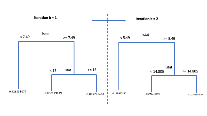
Toy example of gradient boosting
Recall how predictions with GBM are built. We start from the first predicted initial value \(\hat{y}_{i,0}\) , usually set equal to the mean value of the response variable (\(\bar{y}\)). Then we sum up all the the predicted residuals, one for each b iteration,“controlled” for the learning paramenter (\(\sum_{b=0}^{B-1}\lambda * \hat{r}_{i,b}\)). Keep in mind that the first estimated pseudo residual, \(\hat{r}_{i,0}\), corresponds to the first b iteration. In other words, each b estimation of \(y\) is done summing up \(B-1\) pseudo-residuals, starting to count from 0 to B-1. In our case:
- \(\hat{y}_{i,2} = \hat{y}_{i,0} + (\lambda * \hat{r}_{i,0}) + (\lambda * \hat{r}_{i,1})) = \bar{y} +\sum_{b=0}^{B-1}\lambda * \hat{r}_{i,b}\)
Let’s try to compute the first six predictions:
pred <- predict(object=gbm_boston,
                newdata=btest_small,
                n.trees = 2) # compute prediction using both trees
head(btest_small)
## lstat black medv
## 6 5.21 394.12 28.7
## 7 12.43 395.60 22.9
## 9 29.93 386.63 16.5
## 10 17.10 386.71 18.9
## 11 20.45 392.52 15.0
## 12 13.27 396.90 18.9head(pred)## [1] 23.10639 22.86160 22.69601 22.69601 22.69601 22.86160Recall that in the first tree, the threshold value at the first split is \(7.49\). The first observation is the only below this value. Also in the second tree the first observation is below the first split value. In this case, predictions are:
gbm_boston$initF + 0.126433077 + 0.119560280 # initial value + lambda*r_0 + lambda*r_1## [1] 23.10639Observations n. 2 and 6 have the same prediction. Both are included in the right node at the first split, and in the left node in the second split. This is valid in both trees.
gbm_boston$initF + 0.002419849 + (- 0.001219699) # initial value + lambda*r_0 + lambda*r_1## [1] 22.8616Try by yourself to compute predictions for observations 3, 4 and 5!
6.3 Gradient boosting: first run
Now we train a gradient boosting model (gbm) for predicting medv by using all the available regressors. We start by dropping the classification variable, that is not needed anymore:
btrain <- btrain[,-15]
btest <- btest[,-15]
Remember that with gbm there are 3 tuning parameters:
- \(B\) the number of trees (i.e. iterations);
- the learning rate or shrinkage parameter \(\lambda\);
- the maximum depth of each tree \(d\) (interaction depth). Note that more than two splitting nodes are required to detect interactions between variables.
We start by setting \(B=5000\) trees (n.trees = 5000), \(\lambda= 0.1\) (shrinkage = 0.1) and \(d=1\) (interaction.depth = 1, i.e. we consider only stumps). In order to study the effect of the tuning parameter \(B\) we will use 5-folds cross-validation. Given that cross-validation is a random procedure we will set the seed before running the function gbm (see also ?gbm). In order to run the gradient boosting method we will have to specify also distribution = "gaussian":
set.seed(1, sample.kind="Rejection") #we use CV
gbm_boston = gbm(formula = medv ~ .,
                 data = btrain,
                 distribution = "gaussian",
                 n.trees = 5000, #B
                 shrinkage = 0.1, #lambda
                 interaction.depth = 1, #d
                 cv.folds = 5)
We are now interested in exploring the content of the vector cv.error contained in the output object gbm_boston: it contains the values of the cv error (which is an estimate of the test error) for all the values of \(B\) between 1 and 5000. For this reason the length of the vector is equal to \(B\):
length(gbm_boston$cv.error)## [1] 5000We want to discover which is the value of \(B\) for which we obtain the lowest value of the cv error:
min(gbm_boston$cv.error) #lowest value of the cv error## [1] 12.10129which.min(gbm_boston$cv.error) #corresponding value of B## [1] 832The same output could be obtained by using the gbm.perf function. It returns the value of \(B\) (a value included between 1 and 5000) for which the cv error is lowest. Moreover, it provides a plot with the error as a function of the number of iterations: the black line is the training error while the green line is the cv error, the one we are interested in, the blue line indicates the best value of the number of iterations.
gbm.perf(gbm_boston)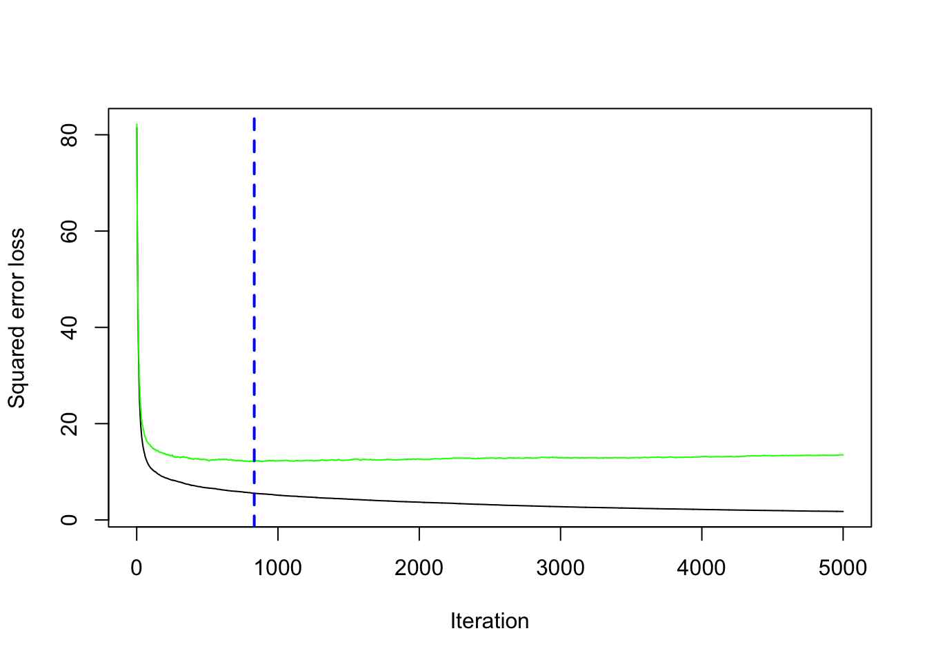
## [1] 8326.4 Gradient boosting: parameter tuning
We have found the best value of \(B\) for two fixed values of \(\lambda\) and \(d\). We have to take into account also possible values for them. In particular, we will consider the value c(0.005, .01, .1) for the learning rate \(\lambda\) and c(1, 3, 5) for the tree depth \(d\). We use a for loop to train 9 gradient boosting algorithms according to the 9 combinations of tuning parameters defined by 3 values of \(\lambda\) combined with 3 values of \(d\). As before, we will use the cv error to choose the best combination of \(\lambda\) and \(d\).
We first create a grid of hyperparameters by using the expand_grid function:
hyper_grid = expand.grid(
  shrinkage = c(0.005, .01, .1),
  interaction.depth = c(1, 3, 5)
)
hyper_grid
## shrinkage interaction.depth
## 1 0.005 1
## 2 0.010 1
## 3 0.100 1
## 4 0.005 3
## 5 0.010 3
## 6 0.100 3
## 7 0.005 5
## 8 0.010 5
## 9 0.100 5class(hyper_grid)## [1] "data.frame"Then we run the for loop with an index i going from 1 to 9 (since 9 are the maximum combinations of hyperparameters). At each iteration of the for loop we use a specific combination of \(\lambda\) and \(d\) taken from hyper_grid. We will finally save the lowest cv error and the corresponding value of \(B\) in new columns of the hyper_grid dataframe:
for(i in 1:nrow(hyper_grid)){

  print(paste("Iteration n.",i))
  set.seed(1, sample.kind="Rejection") #we use CV
  gbm_boston = gbm(formula = medv ~ .,
                   data = btrain,
                   distribution = "gaussian",
                   n.trees = 5000, #B
                   shrinkage = hyper_grid$shrinkage[i], #lambda
                   interaction.depth = hyper_grid$interaction.depth[i], #d
                   cv.folds = 5)

  hyper_grid$minMSE[i] = min(gbm_boston$cv.error)
  hyper_grid$bestB[i] = which.min(gbm_boston$cv.error)
}
## [1] "Iteration n. 1"
## [1] "Iteration n. 2"
## [1] "Iteration n. 3"
## [1] "Iteration n. 4"
## [1] "Iteration n. 5"
## [1] "Iteration n. 6"
## [1] "Iteration n. 7"
## [1] "Iteration n. 8"
## [1] "Iteration n. 9"We see that now hyper_grid contains two additional columns (minMSE and bestB). It is possible to order the data by using the values contained in the minMSE column in order to find the best value of \(\lambda\) and \(d\):
hyper_grid## shrinkage interaction.depth minMSE bestB
## 1 0.005 1 13.397062 5000
## 2 0.010 1 12.554269 4960
## 3 0.100 1 12.101286 832
## 4 0.005 3 9.269789 4992
## 5 0.010 3 8.788457 4891
## 6 0.100 3 8.932166 543
## 7 0.005 5 8.761203 4995
## 8 0.010 5 8.537761 4923
## 9 0.100 5 8.867994 216hyper_grid %>%
arrange(minMSE)## shrinkage interaction.depth minMSE bestB
## 1 0.010 5 8.537761 4923
## 2 0.005 5 8.761203 4995
## 3 0.010 3 8.788457 4891
## 4 0.100 5 8.867994 216
## 5 0.100 3 8.932166 543
## 6 0.005 3 9.269789 4992
## 7 0.100 1 12.101286 832
## 8 0.010 1 12.554269 4960
## 9 0.005 1 13.397062 5000Note that the optimal number of iterations and the learning rate \(\lambda\) depend on each other (the lower the value of \(\lambda\) the higher the number of iterations):
hyper_grid %>%
  arrange(shrinkage)
## shrinkage interaction.depth minMSE bestB
## 1 0.005 1 13.397062 5000
## 2 0.005 3 9.269789 4992
## 3 0.005 5 8.761203 4995
## 4 0.010 1 12.554269 4960
## 5 0.010 3 8.788457 4891
## 6 0.010 5 8.537761 4923
## 7 0.100 1 12.101286 832
## 8 0.100 3 8.932166 543
## 9 0.100 5 8.867994 2166.5 Gradient boosting: final model
Given the best set of hyperparameters, we run the final gbm model with 10000 trees to see if we can get any additional improvement in the cv error.
set.seed(1, sample.kind="Rejection") #we use CV
gbm_final = gbm(formula = medv ~ .,
                 data = btrain,
                 distribution = "gaussian",
                 n.trees = 10000, #B
                 shrinkage = 0.01, #lambda
                 interaction.depth = 5, #d
                 cv.folds = 5)
We save the best value of \(B\) retrieved by using the gbm.perf function in a new object. This will be needed later for prediction:
(bestB = gbm.perf(gbm_final))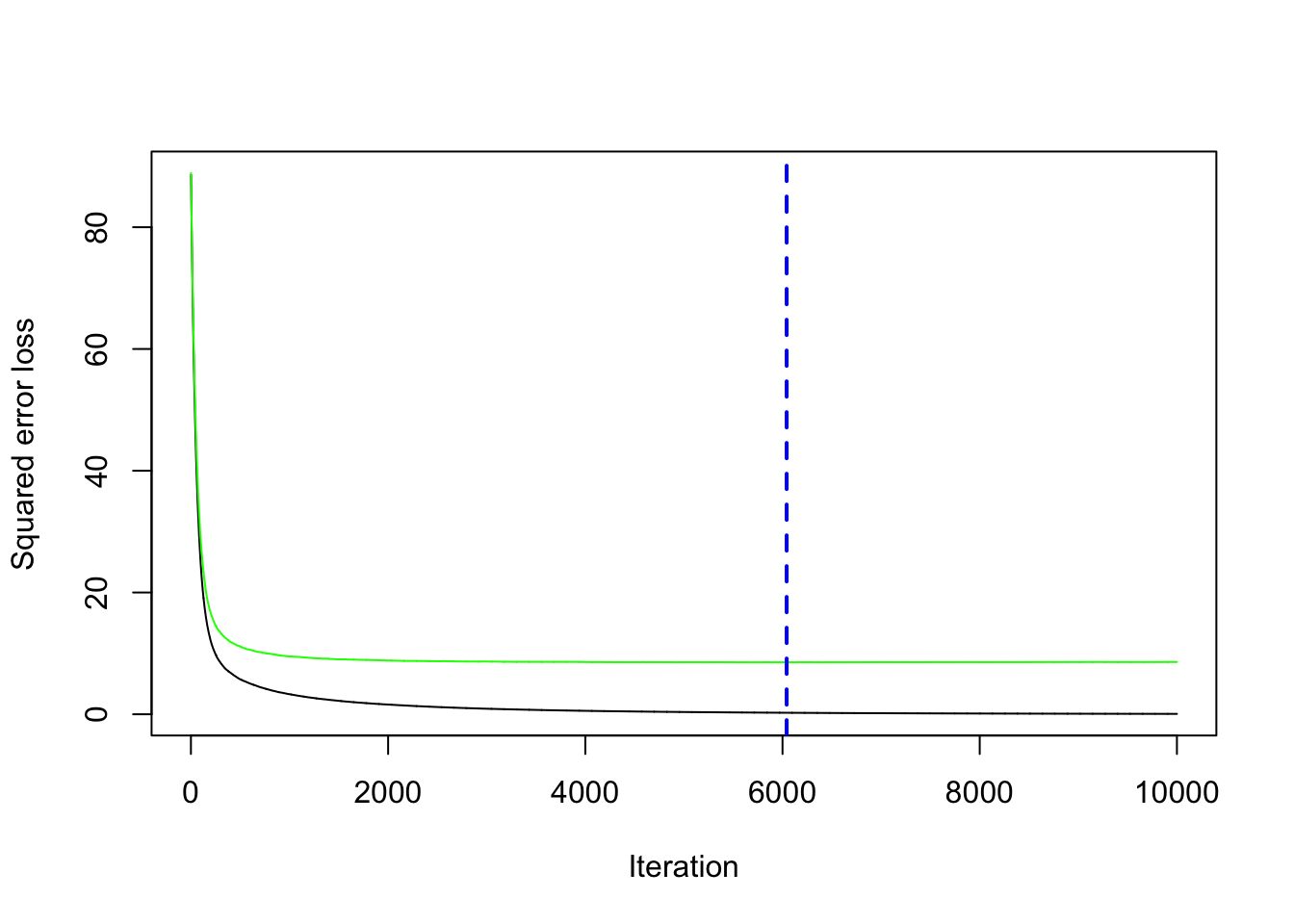
## [1] 6042We compute now the prediction for the test data using the standard predict function for which it will be necessary to specify the value of \(B\) that we want to use (bestB in this case):
pred_boo = predict(gbm_final,
                   btest,
                   n.trees = bestB)
Given the prediction we can compute the MSE:
MSE_boo = mean((btest$medv - pred_boo)^2)
MSE_boo
## [1] 16.38891It is also possible to obtain information about the variable importance in the final model by applying the function summary:
summary(gbm_final)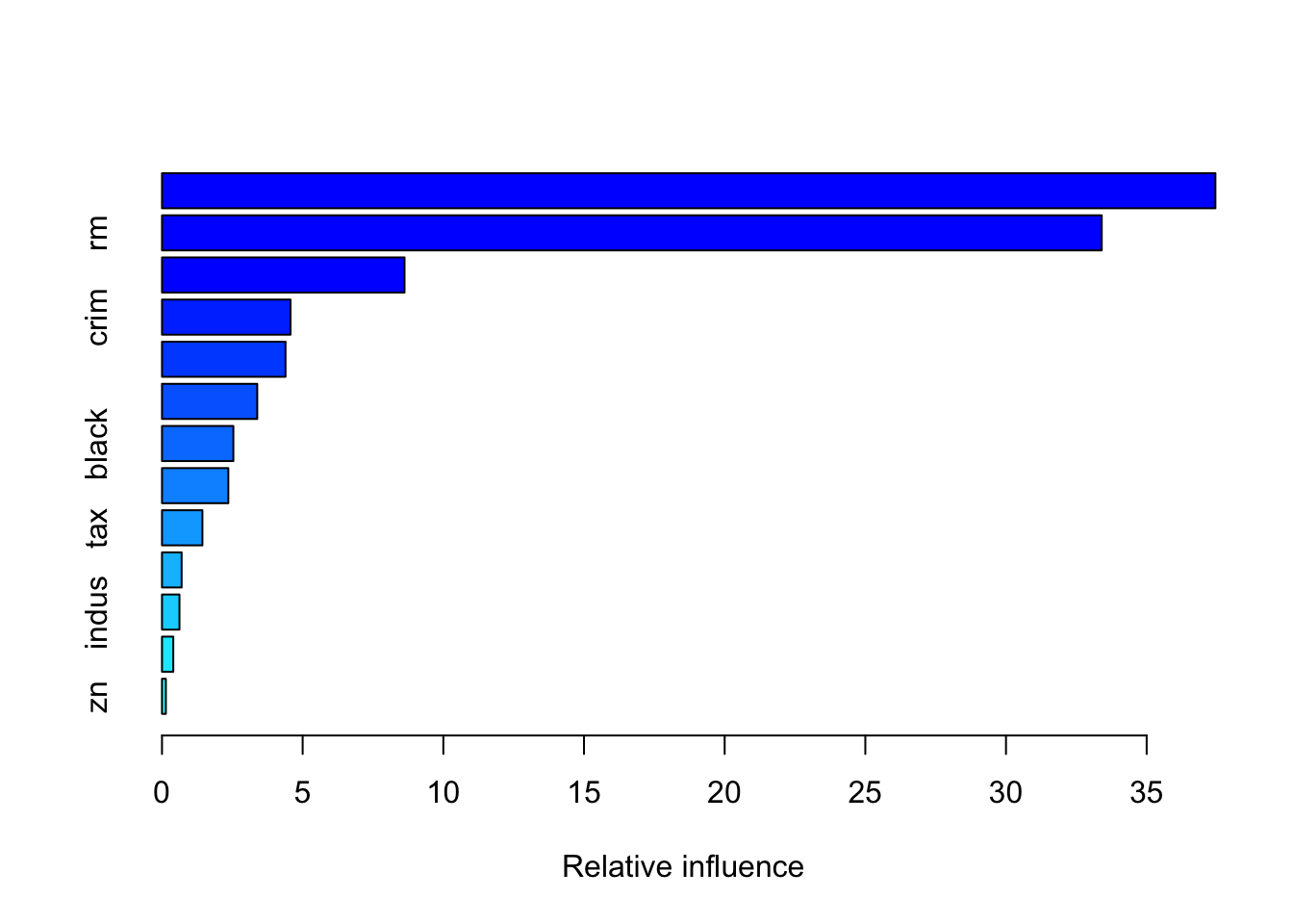
##             var    rel.inf
## lstat     lstat 37.4441271
## rm           rm 33.4032741
## dis         dis  8.6206651
## crim       crim  4.5679984
## nox         nox  4.3908304
## age         age  3.3853064
## black     black  2.5365640
## ptratio ptratio  2.3576062
## tax         tax  1.4367312
## rad         rad  0.6978328
## indus     indus  0.6208496
## chas       chas  0.4013254
## zn           zn  0.1368894
The relative influence of each variable is reported, given the reduction of squared error attributable to each variable. The second column of the output table is the computed relative influence, normalized to sum to 100.
6.6 Linear model, bagging and random forest
As we did before, we are interested in medv (median value of owner-occupied homes in $1000s). We implement first a linear regression model using as regressors all the other variables. Then we compute the predicted value for medv for the test set (btest) and finally compute the test mean square error (we save it in an object called MSE_lm).
lm_boston = linear_reg(engine = 'lm') %>% fit(medv ~ ., data = btrain)
pred_lm = predict(lm_boston, new_data=btest)
MSE_lm = mean((btest$medv - pred_lm$.pred)^2)
MSE_lm
## [1] 17.33601The second alternative method we implement for predicting medv is bagging, described in Section 4.4 and 5.3. As previously done with the linear regression model, we compute the predicted value for medv for the test set (btest) and finally compute the test mean square error (we save it in an object called MSE_bag).
bag_boston = rand_forest(engine = 'randomForest', mode = 'regression',
                         mtry = (ncol(btrain)-1),
                         trees = 1000) %>%
  fit(medv ~ ., data = btrain)
pred_bag = predict(bag_boston, new_data=btest)
MSE_bag = mean((btest$medv - pred_bag$.pred)^2)
MSE_bag
## [1] 14.74978Finally, we implement random forest as described in Section 5.4. We will compare this method with the previous two by using test mean square error (saved in an object called MSE_rf).
rf_boston = rand_forest(engine = 'randomForest', mode = 'regression',
                         mtry = (ncol(btrain)-1)/3,
                         trees = 1000) %>%
  fit(medv ~ ., data = btrain)
pred_rf = predict(rf_boston, new_data=btest)
MSE_rf = mean((btest$medv - pred_rf$.pred)^2)
MSE_rf
## [1] 11.22066By comparing MSE_lm, MSE_bag, MSE_rf and MSE_boo we can identify the best model implemented so far
MSE_lm## [1] 17.33601MSE_bag## [1] 14.74978MSE_rf## [1] 11.22066MSE_boo## [1] 16.38891It results that random forest performs the best because it has the lowest MSE. Even boosting performs poorly than random forest, which is the best method overall.
Given the best method, we can then plot the observed and predicted value of medv and compute the correlation between observed and predicted value (the higher, the better):
plot(btest$medv, pred_rf$.pred)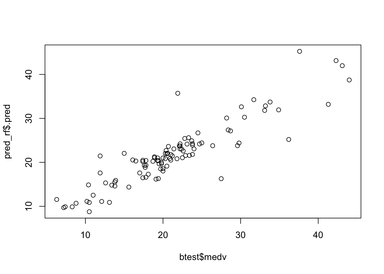
cor(btest$medv, pred_rf$.pred)## [1] 0.90461156.7 Exercises Lab 5
6.7.1 Exercise 1
Consider the bike sharing data used for Lab. 1 (see Section 2.1). Explore the dataset.
The response variable is cnt (count of total rental bikes including both casual and registered users). All the other variables but registered will be used as regressors.
Remove
registeredandcasualfrom the dataframe (ascnt=casual+registered). Remove alsodtedaywhich is a character variable with the date strings.Split the original data set into a training (70%) and test set. Use 44 as seed. Moreove, compute the average number of rental bikes for the two datasets.
Implement bagging to predict
cnt(use 44 as seed and 1000 trees). Compute also the test MSE for bagging.Implement random forest (use 44 as seed) for the same set of data and compare its performance (in terms of MSE) with the method implemented before.
Implement gradient boosting for the same set of data by using \(B=5000\), \(d=1\) and \(\lambda=0.1\) and 5-folds cross-validation. Use 44 as seed.
- Which is the best value of \(B\) for this specific parameter setting?
In order to tune the value of the hyperparameter consider the values
c(0.005, .01, .1, 0.2)for the learning rate \(\lambda\) andc(1, 3, 5, 7)for the tree depth (use \(B=5000\)). Implement a for loop to iterate across the 16 parameters’ combinations. Which is the best setting for \(\lambda\) and \(d\)?Given the parameter values chosen at the previous point, rerun gbm by using \(B=10000\). Then detect the best value of \(B\) and compute the final predictions for the test set and the corresponding MSE.
Compare bagging, random forest and gbm in terms of MSE? Which method does perform better? Study the importance of the variable for the best model.
Given the best method, plot predicted and observed values for
cnt. For setting the color of the points use theseasonvariable.