Chapter 6 R Lab 5 - 12/05/2023
In this lecture we will continue the case study introduced in Section 5. You to run all the code from Lab 4 which includes data preparation starting from the MSFT data.
The following packages are required:
library(tidyverse)
library(lubridate) #for dealing with dates
library(zoo) #for time series manipulating and modeling
library(rpart) #regression/classification tree
library(rpart.plot) #tree plots
library(randomForest) #bagging and random forecast
library(FNN) #for regression KNN
At the end you should have the following two datasets:
glimpse(MSFTtr)## Rows: 1,160
## Columns: 8
## $ Date <date> 2017-05-25, 2017-05-26, 2017-05-30, 2017-05-31, 2017-06-01, 2017-06…
## $ MA2 <dbl> 0.0005927972, 0.0021850423, 0.0042008004, 0.0055389817, 0.0053356564…
## $ MA7 <dbl> 0.0000000000, 0.0001024794, 0.0013126507, 0.0026301730, 0.0036793010…
## $ MA14 <dbl> 0.0000000000, 0.0002496531, 0.0005977847, 0.0010322950, 0.0012602073…
## $ MA21 <dbl> 0.0000000000, 0.0003594390, 0.0007027827, 0.0010892422, 0.0012255786…
## $ SD7 <dbl> 0.05296239, 0.05802160, 0.06711377, 0.07466795, 0.05686829, 0.048740…
## $ lag1volume <dbl> 0.06904779, 0.13898080, 0.11946367, 0.09292550, 0.22164877, 0.136567…
## $ target <dbl> 0.006036340, 0.007553825, 0.005631552, 0.006508324, 0.012106306, 0.0…glimpse(MSFTte)## Rows: 77
## Columns: 8
## $ Date <date> 2022-01-03, 2022-01-04, 2022-01-05, 2022-01-06, 2022-01-07, 2022-01…
## $ MA2 <dbl> 1.0000000, 0.9618317, 0.9007791, 0.7473543, 0.6209897, 0.6014462, 0.…
## $ MA7 <dbl> 0.9960674, 1.0000000, 0.9855889, 0.9194452, 0.8500031, 0.7791910, 0.…
## $ MA14 <dbl> 1.0000000, 0.9925227, 0.9936001, 0.9642216, 0.9465012, 0.9308069, 0.…
## $ MA21 <dbl> 0.9876331, 0.9934102, 1.0000000, 0.9892257, 0.9661175, 0.9431301, 0.…
## $ SD7 <dbl> 0.09785490, 0.06212817, 0.21994156, 0.66243705, 0.88719009, 0.897984…
## $ lag1volume <dbl> 0.0000000, 0.1500012, 0.2025940, 0.3044882, 0.2988522, 0.2032250, 0.…
## $ target <dbl> 1.0000000, 0.7678880, 0.7219434, 0.7248838, 0.7291106, 0.7421593, 0.…Let’s remove the Date from the training dataset because it won’t be used for fitting the model:
MSFTtr = MSFTtr %>% dplyr::select(-Date)6.0.1 Regression tree
We have now the data to estimate the regression tree for predicting the MSFT price, given the 6 selected regressors.
We use now the training data to estimate a regression tree by using the rpart function of the rpart package (see ?rpart). As usual we have to specify the formula, the dataset and the method (which will be set to anova for a regression tree). More information about the anova methodology can be find into this document here (page 32).
singletree = rpart(formula = target ~.,
                  data =  MSFTtr,
                  method = "anova")
Note that some options that control the rpart algorithm are specified by means of the rpart.control function (see ?rpart.control). In particular, the cp option, set by default equal to 0.01, represents a pre-pruning step because it prevents the generation of non-significant branches (any split that does not decrease the overall lack of fit by a factor of cp is not attempted). See also the meaning of the minsplit, minbucket and maxdepth options.
It is possible to plot the estimated tree as follows:
rpart.plot(singletree)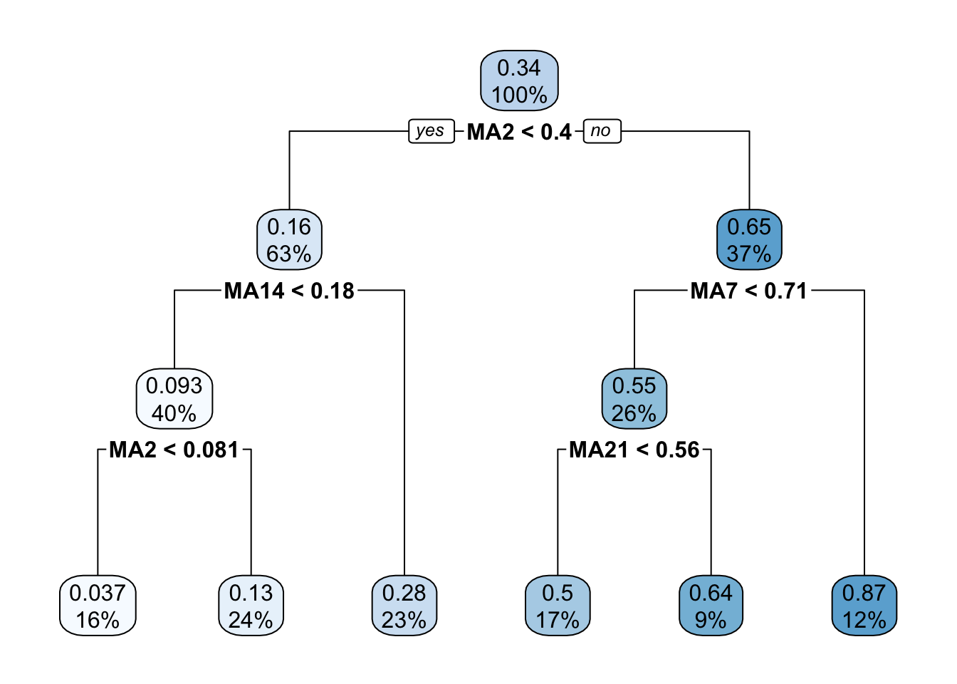
The function rpart.plot has different options about which information should be displayed. Here we use it with its default setting and each node provides the average price and the percentage of training observations in each node (with respect to the total number of training observations). Note that basically all the numbers in the plot are rounded.
It is also possible to analyze the structure of the tree by printing it:
singletree## n= 1160
##
## node), split, n, deviance, yval
## * denotes terminal node
##
## 1) root 1160 84.7423800 0.34201040
## 2) MA2< 0.4017356 729 7.8698120 0.16016720
## 4) MA14< 0.1809473 465 1.2662160 0.09315739
## 8) MA2< 0.0809836 183 0.1166070 0.03702299 *
## 9) MA2>=0.0809836 282 0.1987565 0.12958500 *
## 5) MA14>=0.1809473 264 0.8378773 0.27819590 *
## 3) MA2>=0.4017356 431 11.9938400 0.64958280
## 6) MA7< 0.7050037 296 1.9696930 0.55132710
## 12) MA21< 0.5648444 192 0.4525512 0.50105920 *
## 13) MA21>=0.5648444 104 0.1363078 0.64412940 *
## 7) MA7>=0.7050037 135 0.9008853 0.86501730 *The most important regressor, which is located in the root node, is MA2 (so basically information referring to very few past data).
Given the grown tree we are now able to compute the predictions for the test set and to compute, as measure of performance, the mean squared error (\(MSE = \sum_{i=1}^n(y_i-\hat y_i)^2\) with \(i\) denoting the generic observation in the test set). The predictions can be obtained by using the predict function that will return the vector of predicted prices:
predsingletree = predict(object = singletree,
                    newdata = MSFTte)
# MSE
MSE1tree = mean((MSFTte$target-predsingletree)^2)
MSE1tree
## [1] 0.03220142We also plot the observed test data and the corresponding predictions:
# Define first a data.frame before using ggplot
data.frame(MSFTte, predsingletree) %>%
  ggplot()+
  geom_line(aes(Date,target, col="obs")) +
  geom_line(aes(Date,predsingletree, col="pred1tree"))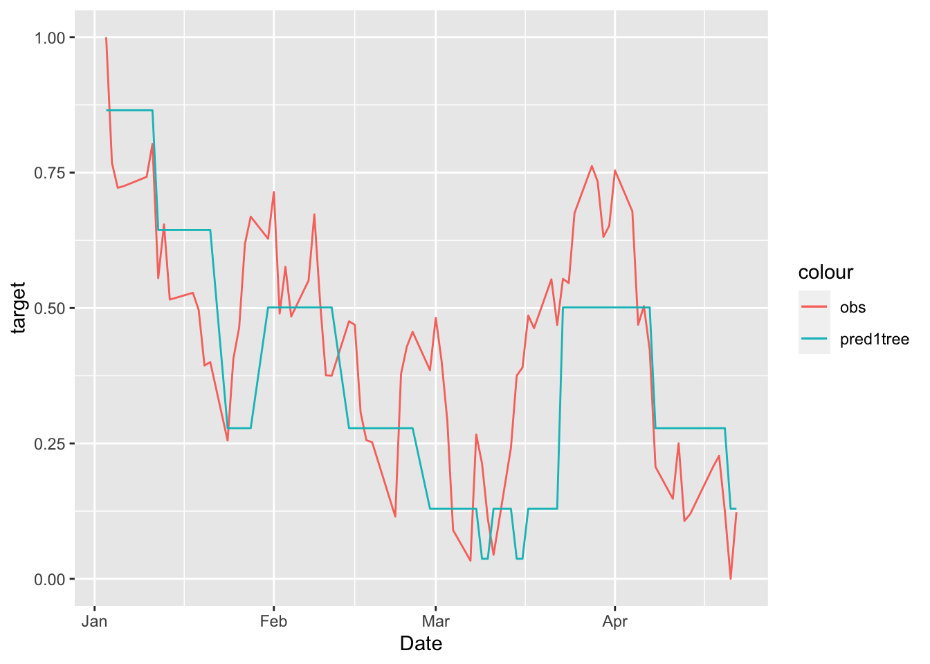
We see that the regression tree is able to get the trend of the test set but it is not doing a good job in the prediction (with many period of constant prediction).
6.1 Pruning
After the estimation of the the decision tree it is possible to remove non-significant branches (pruning) by adopting the cost-complexity approach (i.e. by penalizing for the tree size). To determine the optimal cost-complexity (CP) parameter value \(\alpha\), rpart automatically performs a 10-fold cross validation (see argument xval = 10 in the rpart.control function). The complexity table is part of the standard output of the rpart function and can be obtained as follows:
singletree$cptable## CP nsplit rel error xerror xstd
## 1 0.76559954 0 1.00000000 1.00166420 0.035166329
## 2 0.10765880 1 0.23440046 0.23765846 0.009102505
## 3 0.06803819 2 0.12674166 0.12216520 0.004238147
## 4 0.01629449 3 0.05870347 0.05989170 0.002110345
## 5 0.01122051 4 0.04240898 0.04523947 0.001512709
## 6 0.01000000 5 0.03118847 0.03108513 0.001423453Note that the number of splits is reported, rather than the number of nodes (however remember that the number of final nodes is always given by 1 + the number of splits). The tables reports, for different values of \(\alpha\) (CP) the relative training error (rel.error) and the cross-validation error (xerror) together with its standard error (xstd). Note that the rel.error column is scaled so that the first value is 1.
The usual approach is to select the tree with the lowest cross-validation error (rel error or xerror) and to find the corresponding value of CP and number of splits. In this case we observe the minimum value for nsplit equal to 5, which means 6 regions. This is the full tree estimated before, so in this case pruning is not necessary.
6.2 Bagging
Bagging corresponds to a particular case of random forest when all the regressors are used. For this reason to implement bagging we use the function randomForest in the randomForest package. As the procedure is based on boostrap resampling we need to set the seed. As usual we specify the formula and the data together with the number of regressors to be used (mtry, in this case equal to the number of columns minus the column dedicated to the response variable). The option importance is set to T when we are interested in assessing the importance of the predictors. Finally, ntree represents the number of independent trees to grow (500 is the default value).
As bagging is based on bootstrap which is a random procedure it is convenient to set the seed before running the function:
set.seed(11) #procedure is random (bootstrap)
bagmodel = randomForest(target ~ .,
                   data = MSFTtr,
                   mtry = ncol(MSFTtr)-1,
                   ntree = 1000,
                   importance = TRUE)
Note that the information reported in the output (Mean of squared residuals and % Var explained) are computed using out-of-bag (OOB) observations.
We compute the predictions and the test MSE:
predbag = predict(bagmodel, MSFTte)
MSE_bag = mean((MSFTte$target - predbag)^2)
MSE_bag
## [1] 0.03377854Note that the MSE is slightly higher than the one obtained for the single tree.
We analyze now graphically the importance of the regressors (this output is obtained by setting importance = T):
varImpPlot(bagmodel)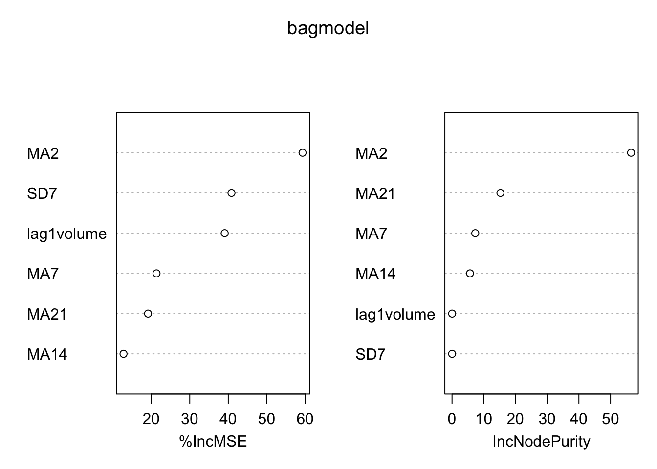
The left plot reports the % increase (averaged across all \(B\) trees) of MSE (computed on the OOB samples) when a given variable is excluded. This measures how much we lose in the predictive capability by excluding each variable. The most important regressor, considering all the \(B\) trees, is MA2.
6.3 Random forest
Random forest is very similar to bagging. The only difference is in the specification
of the mtry argument. For a regression problem we consider a number
of regressors to be selected randomly \(p/3\).
set.seed(11) #procedure is random (bootstrap)
rfmodel = randomForest(target ~ .,
                   data = MSFTtr,
                   mtry = (ncol(MSFTtr)-1) / 3, #p/3
                   ntree = 1000,
                   importance = TRUE)
rfmodel
##
## Call:
## randomForest(formula = target ~ ., data = MSFTtr, mtry = (ncol(MSFTtr) - 1)/3, ntree = 1000, importance = TRUE)
## Type of random forest: regression
## Number of trees: 1000
## No. of variables tried at each split: 2
##
## Mean of squared residuals: 0.0001347537
## % Var explained: 99.82As before we plot the measure for the importance of the regressors:
varImpPlot(rfmodel)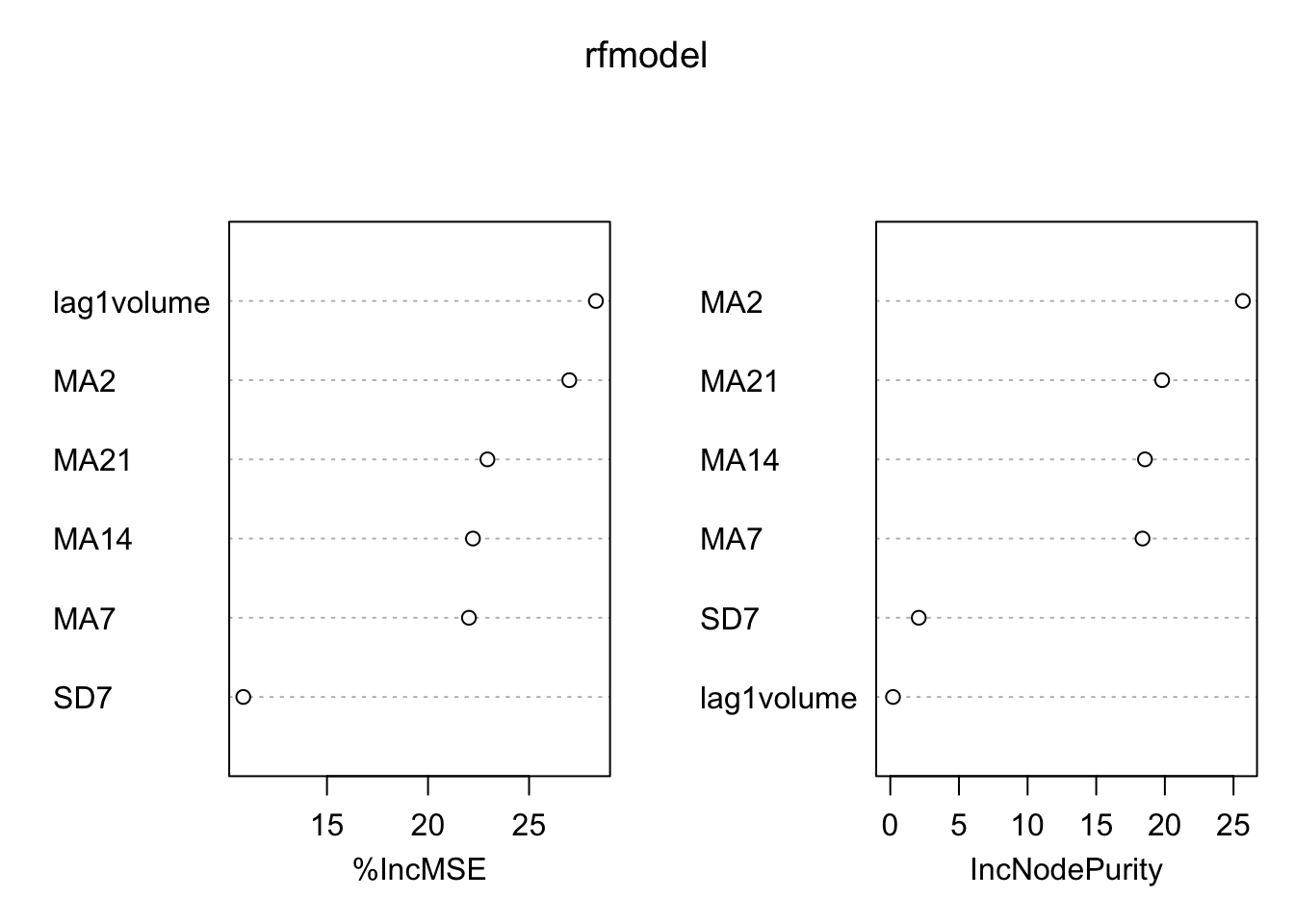 Again
Again MA2 is the most important regressor.
Finally, we compute the predictions and the test MSE by using the random forest model:
predrf = predict(rfmodel, MSFTte)

MSE_rf = mean((MSFTte$target - predrf)^2)
MSE_rf
## [1] 0.0435875It results that random forest is performing worse than bagging. We finally plot all the predictions:
# plot all the predicted time series
data.frame(MSFTte, predsingletree, predbag, predrf) %>%
  ggplot()+
  geom_line(aes(Date,target, col="obs")) +
  geom_line(aes(Date,predsingletree, col="pred1tree")) +
  geom_line(aes(Date,predbag, col="predbag")) +
  geom_line(aes(Date,predrf, col="predrf"))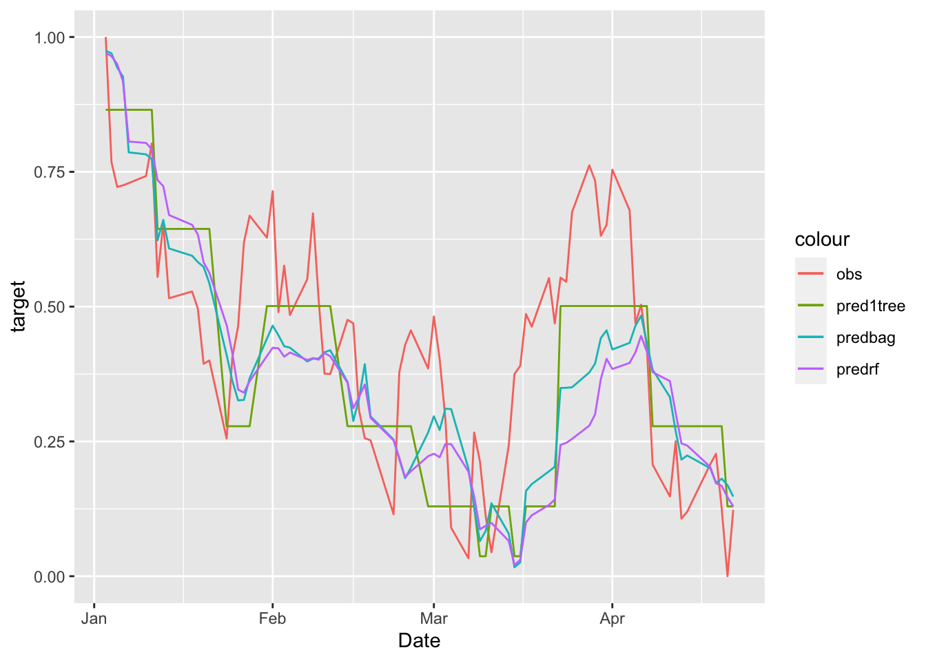
6.4 KNN regression
We finally implemented KNN regression using the FNN library as described in Section 2:
knnmod = knn.reg(train = dplyr::select(MSFTtr, -target),
                 test = dplyr::select(MSFTte, -target, -Date),
                 y = dplyr::select(MSFTtr, target),
                 k = 20) # this is the tuned value of k
# you don't need to run predict
MSE_knn = mean((MSFTte$target - knnmod$pred)^2)
MSE_knn
## [1] 0.045447446.5 Final prediction
We compare the MSEs:
MSE1tree## [1] 0.03220142MSE_bag## [1] 0.03377854MSE_rf## [1] 0.0435875MSE_knn## [1] 0.04544744The method with the lowest MSE is the single regression tree.
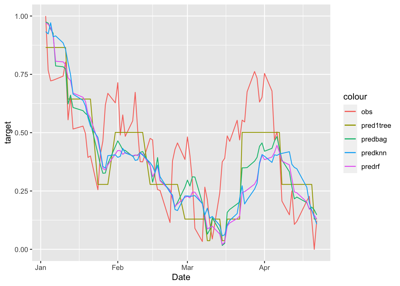
We plot all the predictions together:
data.frame(MSFTte, predsingletree, predbag, predrf, knnmod$pred) %>%
  ggplot()+
  geom_line(aes(Date,target, col="obs")) +
  geom_line(aes(Date,predsingletree, col="pred1tree")) +
  geom_line(aes(Date,predbag, col="predbag")) +
  geom_line(aes(Date,predrf, col="predrf")) +
  geom_line(aes(Date,knnmod.pred, col="predknn"))