Chapter 7 R Lab 6 - 19/05/2023
In this lecture we will learn how to implement gradient boosting (regression). We will also compare the performances of gradient boosting to other regression methods as the linear model and random forest.
The following packages are required: MASS,randomForest, gbm and tidyverse.
library(MASS) # for our dataset
library(tidyverse) # data management
library(randomForest) #for bagging and random forest
library(gbm) #for gradient boosting
We first load the library MASS which contains the dataset Boston (Housing Values in Suburbs of Boston, see ?Boston for the description of the variables). Our response variable would be medv (median value of owner-occupied homes in $1000s), and the others will be used as regressors.
glimpse(Boston)## Rows: 506
## Columns: 14
## $ crim <dbl> 0.00632, 0.02731, 0.02729, 0.03237, 0.06905, 0.02985, 0.08829, 0.14455,…
## $ zn <dbl> 18.0, 0.0, 0.0, 0.0, 0.0, 0.0, 12.5, 12.5, 12.5, 12.5, 12.5, 12.5, 12.5…
## $ indus <dbl> 2.31, 7.07, 7.07, 2.18, 2.18, 2.18, 7.87, 7.87, 7.87, 7.87, 7.87, 7.87,…
## $ chas <int> 0, 0, 0, 0, 0, 0, 0, 0, 0, 0, 0, 0, 0, 0, 0, 0, 0, 0, 0, 0, 0, 0, 0, 0,…
## $ nox <dbl> 0.538, 0.469, 0.469, 0.458, 0.458, 0.458, 0.524, 0.524, 0.524, 0.524, 0…
## $ rm <dbl> 6.575, 6.421, 7.185, 6.998, 7.147, 6.430, 6.012, 6.172, 5.631, 6.004, 6…
## $ age <dbl> 65.2, 78.9, 61.1, 45.8, 54.2, 58.7, 66.6, 96.1, 100.0, 85.9, 94.3, 82.9…
## $ dis <dbl> 4.0900, 4.9671, 4.9671, 6.0622, 6.0622, 6.0622, 5.5605, 5.9505, 6.0821,…
## $ rad <int> 1, 2, 2, 3, 3, 3, 5, 5, 5, 5, 5, 5, 5, 4, 4, 4, 4, 4, 4, 4, 4, 4, 4, 4,…
## $ tax <dbl> 296, 242, 242, 222, 222, 222, 311, 311, 311, 311, 311, 311, 311, 307, 3…
## $ ptratio <dbl> 15.3, 17.8, 17.8, 18.7, 18.7, 18.7, 15.2, 15.2, 15.2, 15.2, 15.2, 15.2,…
## $ black <dbl> 396.90, 396.90, 392.83, 394.63, 396.90, 394.12, 395.60, 396.90, 386.63,…
## $ lstat <dbl> 4.98, 9.14, 4.03, 2.94, 5.33, 5.21, 12.43, 19.15, 29.93, 17.10, 20.45, …
## $ medv <dbl> 24.0, 21.6, 34.7, 33.4, 36.2, 28.7, 22.9, 27.1, 16.5, 18.9, 15.0, 18.9,…We plot the distribution of the response variable medv:
Boston %>%
  ggplot() +
  geom_histogram(aes(medv),col="white")
## `stat_bin()` using `bins = 30`. Pick better value with `binwidth`.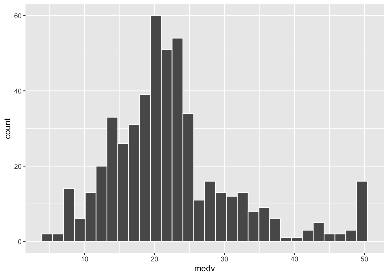
and also the distribution of the response conditionally on the two categories of chas (Charles River dummy variable (= 1 if tract bounds river; 0 otherwise)):
Boston %>%
  ggplot()+
  geom_boxplot(aes(factor(chas), medv))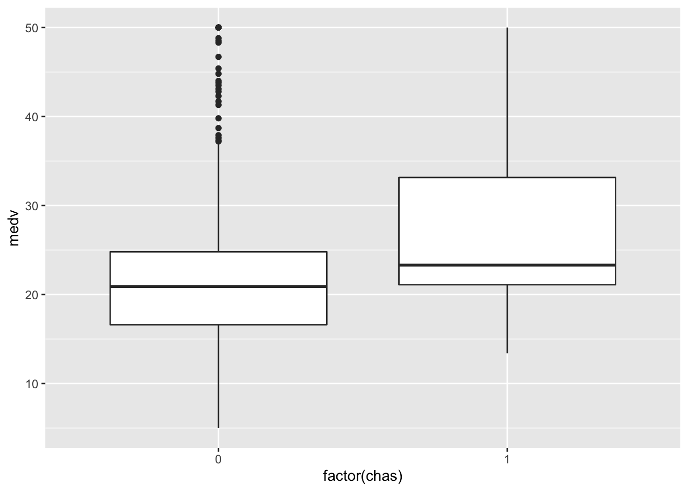
As usual we start by splitting the dataset into two subsets: one for training (called btrain and containing about 80% of the observations) and one for testing (called btest).
set.seed(1)
ind = sample(1:nrow(Boston),
             0.8*nrow(Boston),replace=F)
btrain = Boston[ind,]
btest = Boston[-ind,]
We are now ready to implement the regression models.
7.1 Gradient boosting: first run
Now we train a gradient boosting model (gbm) for predicting medv by using all the available regressors.
Remember that with gbm there are 3 tuning parameters:
- \(B\) the number of trees (i.e. iterations);
- the learning rate or shrinkage parameter \(\lambda\);
- the maximum depth of each tree \(d\) (interaction depth). Note that more than two splitting nodes are required to detect interactions between variables.
We start by setting \(B=5000\) trees (n.trees = 5000), \(\lambda= 0.1\) (shrinkage = 0.1) and \(d=1\) (interaction.depth = 1, i.e. we consider only stumps). In order to study the effect of the tuning parameter \(B\) we will use 5-folds cross-validation. Given that cross-validation is a random procedure we will set the seed before running the function gbm (see also ?gbm). In order to run the gradient boosting method for a regression problem we will have to specify also distribution = "gaussian" (this will use MSE as loss function):
set.seed(1) #we use CV
gbm_boston = gbm(formula = medv ~ .,
                 data = btrain,
                 distribution = "gaussian",
                 n.trees = 5000, #B
                 shrinkage = 0.1, #lambda
                 interaction.depth = 1, #d
                 cv.folds = 5)
We are now interested in exploring the content of the vector cv.error contained in the output object gbm_boston: it contains the values of the cv error (which is an estimate of the test error) for all the values of \(B\) between 1 and 5000. For this reason the length of the vector is equal to \(B\):
length(gbm_boston$cv.error)## [1] 5000We want to discover which is the value of \(B\) for which we obtaine the lowest value of the cv error:
min(gbm_boston$cv.error) #lowest value of the cv error## [1] 12.10129which.min(gbm_boston$cv.error) #corresponding value of B## [1] 832The same output could be obtained by using the gbm.perf function. It returns the value of \(B\) (a value included between 1 and 5000) for which the cv error is lowest. Moreover, it provides a plot with the error as a function of the number of iterations: the black line is the training error while the green line is the cv error, the one we are interested in, the blue line indicates the best value of the number of iterations.
gbm.perf(gbm_boston, method="cv")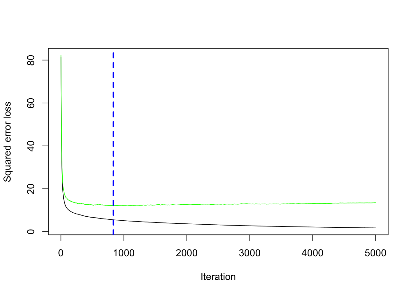
## [1] 8327.2 Gradient boosting: parameter tuning
We have found the best value of \(B\) for two fixed values of \(\lambda\) and \(d\). We have to take into account also possible values for them. In particular, we will consider the value c(0.005, .01, .1) for the learning rate \(\lambda\) and c(1, 3, 5) for the tree depth \(d\). We use a for loop to train 9 gradient boosting algorithms according to the 9 combinations of tuning parameters defined by 3 values of \(\lambda\) combined with 3 values of \(d\). As before, we will use the cv error to choose the best combination of \(\lambda\) and \(d\).
We first create a grid of hyperparameters by using the expand_grid function:
grid = expand.grid(
  lambda = c(0.005, .01, .1),
  d = c(1, 3, 5)
)
grid
## lambda d
## 1 0.005 1
## 2 0.010 1
## 3 0.100 1
## 4 0.005 3
## 5 0.010 3
## 6 0.100 3
## 7 0.005 5
## 8 0.010 5
## 9 0.100 5class(grid)## [1] "data.frame"Then we run the for loop with an index i going from 1 to 9 (since 9 are the maximum combinations of hyperparameters). At each iteration of the for loop we use a specific combination of \(\lambda\) and \(d\) taken from grid. We also create two new columns filled with NA where we will save the lowest cv error and the corresponding value of \(B\):
grid$bestB = NA
grid$cverror = NAfor(i in 1:nrow(grid)){
print(paste("Iteration n.",i))
set.seed(1) #we use CV
gbm_boston = gbm(formula = medv ~ .,
data = btrain,
distribution = "gaussian",
n.trees = 5000, #B
shrinkage = grid$lambda[i],
interaction.depth = grid$d[i],
cv.folds = 5)
grid$bestB[i] = min(gbm_boston$cv.error)
grid$cverror[i] = which.min(gbm_boston$cv.error)
}## [1] "Iteration n. 1"
## [1] "Iteration n. 2"
## [1] "Iteration n. 3"
## [1] "Iteration n. 4"
## [1] "Iteration n. 5"
## [1] "Iteration n. 6"
## [1] "Iteration n. 7"
## [1] "Iteration n. 8"
## [1] "Iteration n. 9"Check now grid and see that the last two columns contain some values:
grid## lambda d bestB cverror
## 1 0.005 1 13.397062 5000
## 2 0.010 1 12.554269 4960
## 3 0.100 1 12.101286 832
## 4 0.005 3 9.269789 4992
## 5 0.010 3 8.788457 4891
## 6 0.100 3 8.932166 543
## 7 0.005 5 8.761203 4995
## 8 0.010 5 8.537761 4923
## 9 0.100 5 8.867994 216It is possible to order the data by using the values contained in the cverror column in order to find the best value of \(\lambda\) and \(d\):
grid %>% arrange(cverror)## lambda d bestB cverror
## 1 0.100 5 8.867994 216
## 2 0.100 3 8.932166 543
## 3 0.100 1 12.101286 832
## 4 0.010 3 8.788457 4891
## 5 0.010 5 8.537761 4923
## 6 0.010 1 12.554269 4960
## 7 0.005 3 9.269789 4992
## 8 0.005 5 8.761203 4995
## 9 0.005 1 13.397062 5000Note that the optimal number of iterations and the learning rate \(\lambda\) depend on each other (the lower the value of \(\lambda\) the higher the number of iterations):
grid %>% arrange(d)## lambda d bestB cverror
## 1 0.005 1 13.397062 5000
## 2 0.010 1 12.554269 4960
## 3 0.100 1 12.101286 832
## 4 0.005 3 9.269789 4992
## 5 0.010 3 8.788457 4891
## 6 0.100 3 8.932166 543
## 7 0.005 5 8.761203 4995
## 8 0.010 5 8.537761 4923
## 9 0.100 5 8.867994 2167.3 Gradient boosting: final model
Given the best set of hyperparameters, we run the final gbm model with 7000 trees (to see if we can get any additional improvement in the cv error).
set.seed(1, sample.kind="Rejection") #we use CV
gbm_final = gbm(formula = medv ~ .,
                 data = btrain,
                 distribution = "gaussian",
                 n.trees = 7000, #B
                 shrinkage = 0.01, #lambda
                 interaction.depth = 5, #d
                 cv.folds = 5)
We save the best value of \(B\) retrieved by using the gbm.perf function in a new object. This will be needed later for prediction:
bestB = gbm.perf(gbm_final, method="cv")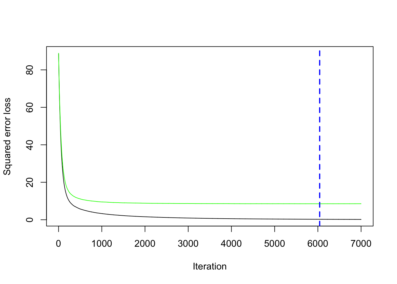
We compute now the prediction for the test data using the standard predict function for which it will be necessary to specify the value of \(B\) that we want to use (bestB in this case):
pred_gbm = predict(gbm_boston,
                   btest,
                   n.trees = bestB)
## Warning in predict.gbm(gbm_boston, btest, n.trees = bestB): Number of trees not specified
## or exceeded number fit so far. Using 5000.Given the prediction we can compute the MSE:
MSE_gbm = mean((btest$medv - pred_gbm)^2)
MSE_gbm
## [1] 17.92962It is also possible to obtain information about the variable importance in the final model by applying the function summary:
summary(gbm_final)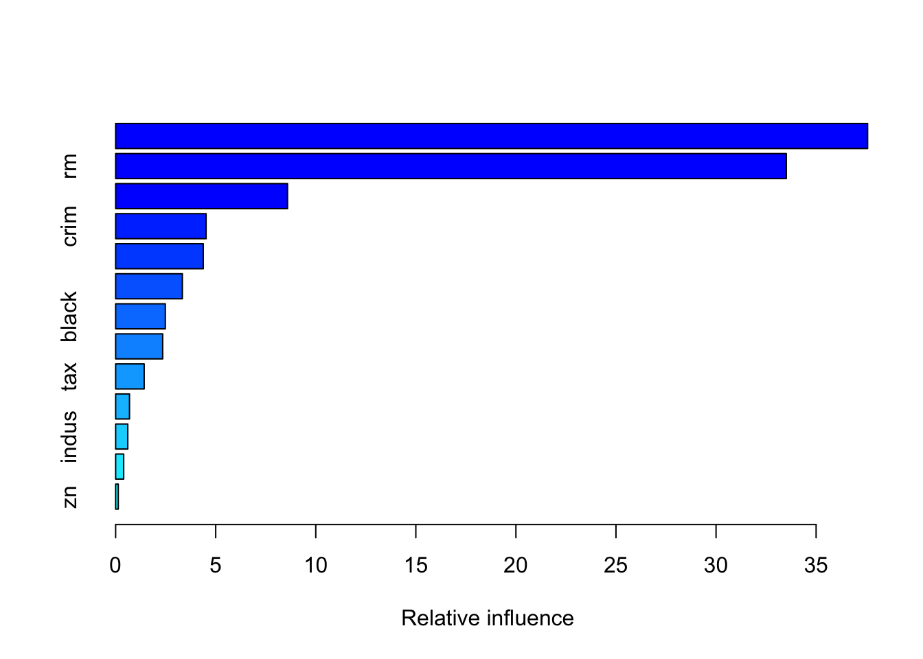
##             var    rel.inf
## lstat     lstat 37.5738986
## rm           rm 33.5111520
## dis         dis  8.5897174
## crim       crim  4.5199865
## nox         nox  4.3790091
## age         age  3.3337262
## black     black  2.4824537
## ptratio ptratio  2.3509476
## tax         tax  1.4258556
## rad         rad  0.6926768
## indus     indus  0.6065156
## chas       chas  0.4028178
## zn           zn  0.1312431
The relative influence of each variable is reported, given the reduction of squared error attributable to each variable. The second column of the output table is the computed relative influence, normalized to sum to 100.
7.4 Linear model, bagging and random forest
As we did before, we are interested in medv (median value of owner-occupied homes in $1000s). We implement first a linear regression model using as regressors all the other variables. Then we compute the predicted value for medv for the test set (btest) and finally compute the test mean square error (we save it in an object called MSE_lm).
lm_boston = lm(medv ~ ., data=btrain)
pred_lm = predict(lm_boston, newdata=btest)
MSE_lm = mean((btest$medv - pred_lm)^2)
MSE_lm
## [1] 17.33601The second alternative method we implement for predicting medv is random forest as described in Section ??. We will compare this method with the previous two by using test mean square error (saved in an object called MSE_rf).
rf_boston = randomForest(formula = medv ~ .,
                         data = btrain,
                         mtry = (ncol(btrain)-1)/3,
                         importance = T,
                         ntree = 1000)
pred_rf = predict(rf_boston, newdata=btest)
MSE_rf = mean((btest$medv - pred_rf)^2)
MSE_rf
## [1] 11.24745By comparing MSE_lm, MSE_rf and MSE_gbm we can identify the best model implemented so far
MSE_lm## [1] 17.33601MSE_rf## [1] 11.24745MSE_gbm## [1] 17.92962It results that random forest performs the best because it has the lowest MSE. Even boosting performs poorly than random forest, which is the best method overall.
Given the best method, we can then plot the observed and predicted value of medv
# FAST plot
data.frame(obs=btest$medv,
           pred_lm,
           pred_rf,
           pred_gbm) %>%
  ggplot()+
  geom_point(aes(obs,pred_gbm,col="boo")) +
  geom_point(aes(obs,pred_rf,col="rf"))+
  geom_point(aes(obs,pred_lm,col="lm"))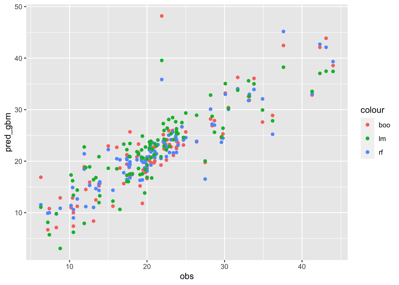
# ELEGANT PLOT with long data
data.frame(obs=btest$medv,
           pred_lm,
           pred_rf,
           pred_gbm) %>%
  pivot_longer(pred_lm:pred_gbm) %>%
  ggplot()+
  geom_point(aes(obs,value,col=name)) +
  facet_wrap(~name) +
  geom_abline(intercept=0, slope=1)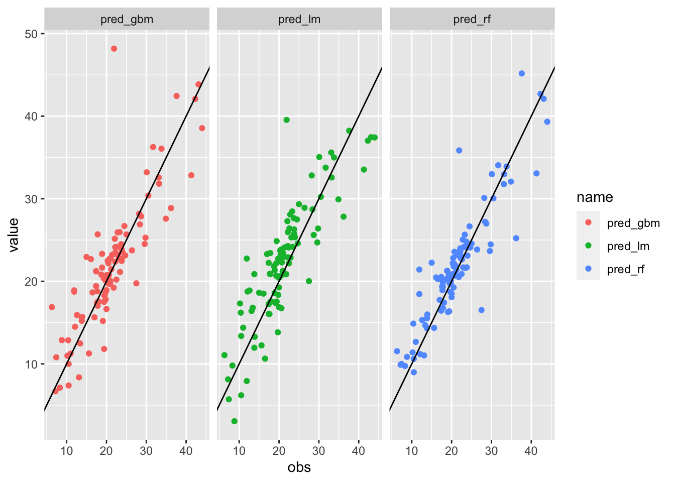
We can also compute the correlation between observed and predicted value (the higher, the better):
# FAST WAY
cor(btest$medv, pred_lm)
## [1] 0.859714cor(btest$medv, pred_rf)## [1] 0.904555cor(btest$medv, pred_gbm)## [1] 0.8515605# ELEGANT WAY WITH LONG DATA
data.frame(obs=btest$medv,
pred_lm,
pred_rf,
pred_gbm) %>%
pivot_longer(pred_lm:pred_gbm) %>%
group_by(name) %>%
summarise(cor(obs,value))## # A tibble: 3 × 2
## name `cor(obs, value)`
## <chr> <dbl>
## 1 pred_gbm 0.852
## 2 pred_lm 0.860
## 3 pred_rf 0.905