Chapter 4 R Lab 3 - 28/04/2023
In this lecture we will learn how to implement:
- the logistic regression model
- LDA and QDA
- Naive Bayes
All the methods will be compared by using performance indexes and the ROC curve. In particular, we will use the following our own function named perf_indexes for computing sensitivity, specificity and accuracy (it takes as input the confusion matrix):
perf_indexes = function(cf){
  accuracy = sum(diag(cf))/sum(cf)
  sensitivity = cf[2,2] / (cf[1,2]+cf[2,2])
  specificity = cf[1,1] / (cf[1,1]+cf[2,1])
  return(c(acc=accuracy, sens=sensitivity, spec=specificity))
}
The following packages are required:
library(tidyverse)
library(MASS) #for lda and qda
library(pROC) #for the ROC curve
library(naivebayes) #for Naive Bayes
4.1 Diabetes data
The data we use for this lab are from the Kaggle platform link. The objective of the analysis is to predict whether or not a patient has diabetes, based on certain diagnostic measurements.
The datasets consists of several predictor variables:
Pregnancies: Number of pregnanciesGlucose: Plasma glucose concentration a 2 hours in an oral glucose tolerance testBloodPressure: Diastolic blood pressure (mm Hg)SkinThickness: Triceps skin fold thickness (mm)Insulin: 2-Hour serum insulin (mu U/ml)BMI: Body mass index (weight in kg/(height in m)^2)DiabetesPedigreeFunction: Diabetes pedigree functionAge: Age (years)
The response variable is named Outcome and is a binary variable: 0 means that the patient does not have diabetes, while 1 means the patient does have diabetes.
We import the data
diabetes <- read.csv("./files/diabetes.csv")
glimpse(diabetes)
## Rows: 768
## Columns: 9
## $ Pregnancies <int> 6, 1, 8, 1, 0, 5, 3, 10, 2, 8, 4, 10, 10, 1, 5, 7, 0, …
## $ Glucose <int> 148, 85, 183, 89, 137, 116, 78, 115, 197, 125, 110, 16…
## $ BloodPressure <int> 72, 66, 64, 66, 40, 74, 50, 0, 70, 96, 92, 74, 80, 60,…
## $ SkinThickness <int> 35, 29, 0, 23, 35, 0, 32, 0, 45, 0, 0, 0, 0, 23, 19, 0…
## $ Insulin <int> 0, 0, 0, 94, 168, 0, 88, 0, 543, 0, 0, 0, 0, 846, 175,…
## $ BMI <dbl> 33.6, 26.6, 23.3, 28.1, 43.1, 25.6, 31.0, 35.3, 30.5, …
## $ DiabetesPedigreeFunction <dbl> 0.627, 0.351, 0.672, 0.167, 2.288, 0.201, 0.248, 0.134…
## $ Age <int> 50, 31, 32, 21, 33, 30, 26, 29, 53, 54, 30, 34, 57, 59…
## $ Outcome <int> 1, 0, 1, 0, 1, 0, 1, 0, 1, 1, 0, 1, 0, 1, 1, 1, 1, 1, …We transform this 0/1 response variable into a factor with categories “No” and “Yes”:
diabetes %>% count(Outcome)## Outcome n
## 1 0 500
## 2 1 268diabetes$Outcome = factor(diabetes$Outcome, labels=c("No", "Yes"))
diabetes %>% count(Outcome)## Outcome n
## 1 No 500
## 2 Yes 268Some exploratory analysis can be done to study the distribution of the regressors conditionally on the diabetes condition. We consider here, as an example, BMI or Pregnancies:
diabetes %>%
  ggplot() +
  geom_boxplot(aes(BMI,fill=Outcome))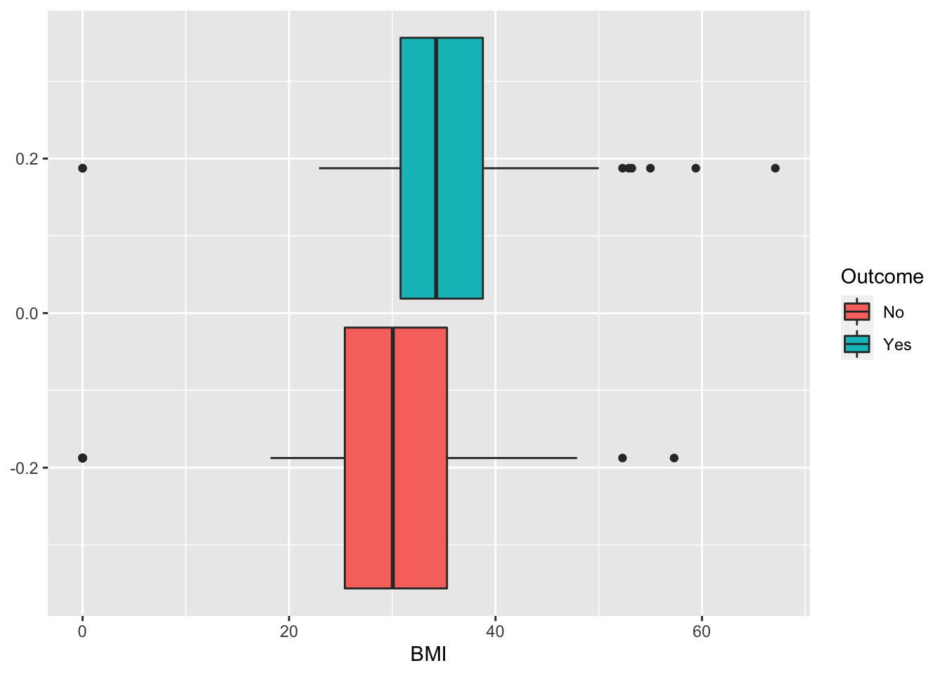
diabetes %>%
  ggplot() +
  geom_density(aes(Pregnancies,fill=Outcome),alpha=0.3)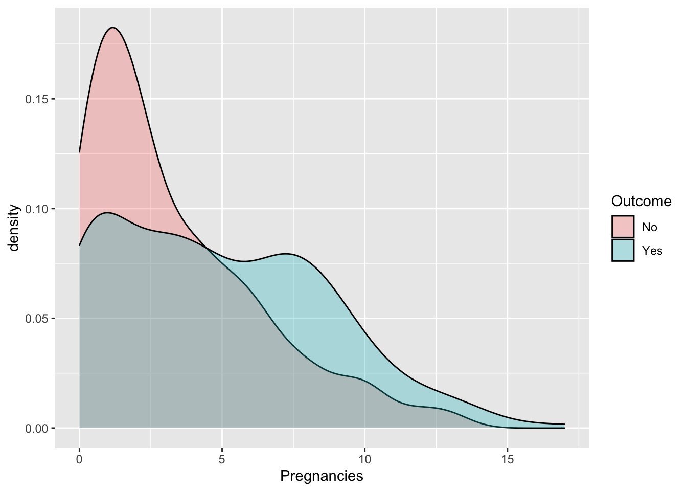
We create the training (70%) and test (30%) data as described in Section 3.3:
set.seed(5)
#Create training set
# positions of the training data
training_index = sample(1:nrow(diabetes),
                        nrow(diabetes)*.7, replace=F)
head(training_index)
## [1] 697 207 715 725 222 71d_train = diabetes[training_index , ]
d_test = diabetes[- training_index , ]
glimpse(d_train)## Rows: 537
## Columns: 9
## $ Pregnancies <int> 3, 8, 3, 1, 2, 2, 6, 5, 5, 3, 1, 0, 1, 8, 5, 6, 7, 2, …
## $ Glucose <int> 169, 196, 102, 111, 158, 100, 0, 136, 116, 116, 118, 1…
## $ BloodPressure <int> 74, 76, 74, 94, 90, 66, 68, 84, 74, 74, 58, 80, 54, 86…
## $ SkinThickness <int> 19, 29, 0, 0, 0, 20, 41, 41, 29, 15, 36, 37, 0, 0, 0, …
## $ Insulin <int> 125, 280, 0, 0, 0, 90, 0, 88, 0, 105, 94, 210, 0, 0, 0…
## $ BMI <dbl> 29.9, 37.5, 29.5, 32.8, 31.6, 32.9, 39.0, 35.0, 32.3, …
## $ DiabetesPedigreeFunction <dbl> 0.268, 0.605, 0.121, 0.265, 0.805, 0.867, 0.727, 0.286…
## $ Age <int> 31, 57, 32, 45, 66, 28, 41, 35, 35, 24, 23, 23, 62, 22…
## $ Outcome <fct> Yes, Yes, No, No, Yes, Yes, Yes, Yes, Yes, No, No, No,…glimpse(d_test)## Rows: 231
## Columns: 9
## $ Pregnancies <int> 0, 2, 4, 10, 10, 1, 5, 7, 1, 1, 3, 9, 13, 3, 9, 3, 7, …
## $ Glucose <int> 137, 197, 110, 168, 139, 189, 166, 107, 103, 115, 126,…
## $ BloodPressure <int> 40, 70, 92, 74, 80, 60, 72, 74, 30, 70, 88, 80, 82, 58…
## $ SkinThickness <int> 35, 45, 0, 0, 0, 23, 19, 0, 38, 30, 41, 35, 19, 11, 37…
## $ Insulin <int> 168, 543, 0, 0, 0, 846, 175, 0, 83, 96, 235, 0, 110, 5…
## $ BMI <dbl> 43.1, 30.5, 37.6, 38.0, 27.1, 30.1, 25.8, 29.6, 43.3, …
## $ DiabetesPedigreeFunction <dbl> 2.288, 0.158, 0.191, 0.537, 1.441, 0.398, 0.587, 0.254…
## $ Age <int> 33, 53, 30, 34, 57, 59, 51, 31, 33, 32, 27, 29, 57, 22…
## $ Outcome <fct> Yes, Yes, No, Yes, No, Yes, Yes, Yes, No, Yes, No, Yes…4.2 Logistic regression
For implementing the logistic regression the function glm (generalized linear model) is used. It requires the specification of the formula, of the dataframe containing the training data and of the distribution (family) of the response variable (in this case binomial distribution given that we are working with a binary response):
logreg = glm(Outcome ~ .,
            data = d_train,
            family = "binomial")
summary(logreg)
##
## Call:
## glm(formula = Outcome ~ ., family = "binomial", data = d_train)
##
## Deviance Residuals:
## Min 1Q Median 3Q Max
## -2.6837 -0.7303 -0.3920 0.7382 2.8346
##
## Coefficients:
## Estimate Std. Error z value Pr(>|z|)
## (Intercept) -9.0648469 0.8905305 -10.179 < 2e-16 ***
## Pregnancies 0.0965714 0.0378905 2.549 0.01081 *
## Glucose 0.0336503 0.0042999 7.826 5.05e-15 ***
## BloodPressure -0.0096448 0.0061956 -1.557 0.11954
## SkinThickness 0.0004596 0.0084002 0.055 0.95637
## Insulin -0.0007987 0.0011917 -0.670 0.50272
## BMI 0.1045459 0.0187457 5.577 2.45e-08 ***
## DiabetesPedigreeFunction 1.2124713 0.3851011 3.148 0.00164 **
## Age 0.0171259 0.0113029 1.515 0.12973
## ---
## Signif. codes: 0 '***' 0.001 '**' 0.01 '*' 0.05 '.' 0.1 ' ' 1
##
## (Dispersion parameter for binomial family taken to be 1)
##
## Null deviance: 702.55 on 536 degrees of freedom
## Residual deviance: 501.28 on 528 degrees of freedom
## AIC: 519.28
##
## Number of Fisher Scoring iterations: 5Note that the notation Outcome ~. means that all the covariates but Outcome are included as regressors (this avoids to write the formula in the standard way: Outcome ~ Pregnancies+Glucose+...).
The summary contains the parameter estimates and the corresponding p-values of the test checking \(H_0:\beta =0\) vs \(H_1: \beta\neq 0\). Consider for example the parameter of the Pregnancies variable which is positive (i.e. higher risk of diabetes) and equal to 0.0965714: this means that for a one-unit increase in the number of pregnancies, the log-odds increases by 0.0965714. For a simpler interpretation, in the odds scale, we can take the exponential transformation of the parameter:
exp(logreg$coefficients[2])## Pregnancies
## 1.101388This means that for a one-unit increase in the number of pregnancies, we expect a 10.14 increase in the diabetes odds (remember that the odds is strictly connected to the diabetes probability as it is defined as \(p/(1-p)\)).
We are now interested in computing predictions for the test observations given the estimated logistic model. They can be obtained by using the predict function. It is important to specify that we are interested in the prediction on the outcome scale (otherwise we will get the predictions on the logit scale):
logreg_pred = predict.glm(logreg,
                          newdata = d_test,
                          type = "response")
head(logreg_pred)
## 5 9 11 12 13 14
## 0.9471784 0.7225479 0.2336053 0.8855958 0.7962820 0.6873194The object logreg_pred contains the conditional probability of having diabetes given the covariate vector. For example for the first test observation the diabetes probability is equal to logreg_pred[1]. In order to have a categorical prediction it is necessary to fix a threshold for the probability (default is 0.5) and transform correspondingly the probabilities:
logreg_pred2 = ifelse(logreg_pred > 0.5, "Yes", "No")
head(logreg_pred2)
## 5 9 11 12 13 14
## "Yes" "Yes" "No" "Yes" "Yes" "Yes"As expected, the predicted category for the first observation is “Yes”.
We are now ready to compute the confusion matrix
table(pred=logreg_pred2, obs=d_test$Outcome)## obs
## pred No Yes
## No 136 33
## Yes 21 41and the performance index by using the function we defined previously and named perf_indexes:
perf_indexes(table(pred=logreg_pred2, obs=d_test$Outcome))## acc sens spec
## 0.7662338 0.5540541 0.8662420Note that the sensitivity is quite low.
4.3 Linear and quadratic discriminant analysis
To run LDA we use the lda function of the MASS package. Similarly to logistic regression we have to specify the formula and the data:
ldaout = lda(Outcome ~ ., data = d_train)
ldaout
## Call:
## lda(Outcome ~ ., data = d_train)
##
## Prior probabilities of groups:
## No Yes
## 0.6387337 0.3612663
##
## Group means:
## Pregnancies Glucose BloodPressure SkinThickness Insulin BMI
## No 3.314869 110.4402 68.62099 19.69388 65.05831 30.00525
## Yes 4.788660 142.8093 72.58763 23.35567 100.12371 35.39948
## DiabetesPedigreeFunction Age
## No 0.4246793 31.30321
## Yes 0.5515412 37.28866
##
## Coefficients of linear discriminants:
## LD1
## Pregnancies 0.0715037089
## Glucose 0.0247199682
## BloodPressure -0.0075594058
## SkinThickness 0.0007927515
## Insulin -0.0003699539
## BMI 0.0673938364
## DiabetesPedigreeFunction 0.8120890336
## Age 0.0129129676The output reports the prior probabilities for the two categories and the conditional means of all the covariates.
We go straight to the calculation of the predictions:
lda_pred = predict(ldaout, newdata = d_test)
names(lda_pred)
## [1] "class" "posterior" "x"Note that the object lda_pred is a list containing 3 objects including the vector of posterior probabilities (posterior) and the vector of predicted categories (`class):
head(lda_pred$posterior)## No Yes
## 5 0.0627473 0.9372527
## 9 0.2277318 0.7722682
## 11 0.7885575 0.2114425
## 12 0.1184079 0.8815921
## 13 0.2056641 0.7943359
## 14 0.2475841 0.7524159head(lda_pred$class)## [1] Yes Yes No Yes Yes Yes
## Levels: No YesTo compute the confusion matrix we will use the vector lda_pred$class:
table(pred=lda_pred$class, obs=d_test$Outcome)## obs
## pred No Yes
## No 137 33
## Yes 20 41perf_indexes(table(pred=lda_pred$class, obs=d_test$Outcome))## acc sens spec
## 0.7705628 0.5540541 0.8726115For the quadratic discriminant analysis everything is very similar except the use of the function qda instead of lda:
qdaout = qda(Outcome ~ ., data = d_train)
qdaout
## Call:
## qda(Outcome ~ ., data = d_train)
##
## Prior probabilities of groups:
## No Yes
## 0.6387337 0.3612663
##
## Group means:
## Pregnancies Glucose BloodPressure SkinThickness Insulin BMI
## No 3.314869 110.4402 68.62099 19.69388 65.05831 30.00525
## Yes 4.788660 142.8093 72.58763 23.35567 100.12371 35.39948
## DiabetesPedigreeFunction Age
## No 0.4246793 31.30321
## Yes 0.5515412 37.28866# predictions
qda_pred = predict(qdaout, newdata = d_test)
names(qda_pred)## [1] "class" "posterior"head(qda_pred$class)## [1] Yes Yes No Yes Yes Yes
## Levels: No Yeshead(qda_pred$posterior)## No Yes
## 5 1.968997e-04 0.9998031
## 9 9.971334e-05 0.9999003
## 11 8.131565e-01 0.1868435
## 12 3.347308e-02 0.9665269
## 13 8.658818e-02 0.9134118
## 14 6.217003e-10 1.0000000perf_indexes(table(pred=qda_pred$class, obs=d_test$Outcome))## acc sens spec
## 0.7316017 0.5270270 0.8280255Also for LDA and QDA the sensitivity is low.
4.4 Naive Bayes
The function naive_bayes from the naivebayes package is used to implement the Naive Bayes algorithm which is based on the Bayes’ algorithm:
nbout = naive_bayes(Outcome ~ .,
                   data = d_train,
                    usekernel = TRUE)
summary(nbout)
##
## ======================================= Naive Bayes ========================================
##
## - Call: naive_bayes.formula(formula = Outcome ~ ., data = d_train, usekernel = TRUE)
## - Laplace: 0
## - Classes: 2
## - Samples: 537
## - Features: 8
## - Conditional distributions:
## - KDE: 8
## - Prior probabilities:
## - No: 0.6387
## - Yes: 0.3613
##
## --------------------------------------------------------------------------------------------Note that the option usekernel = TRUE is used in order to estimate the density \(\hat f_{jk}\) (for covariate \(X_j\) in category \(k\)) by using the kernel density estimate (smoothed version of the histogram).
We move on by computing predictions, as done with the previous methods:
nb_pred = predict(nbout, d_test)## Warning: predict.naive_bayes(): more features in the newdata are provided as there are
## probability tables in the object. Calculation is performed based on features to be found
## in the tables.head(nb_pred)## [1] Yes Yes No Yes Yes Yes
## Levels: No YesThe warning message that we get is not important (it is just saying that in the test dataset there are additional variables that weren’t used as regressors in the training, in this case it is reffering to charged_off which is actually our response variable). Note that in this case nbmodpred is not a list (as with LDA and QDA) but a vector of the predicted categories (not the probabilities). If you are interested in the posterior probabilities run the following code (you will need these probabilities when computing the ROC curve):
nb_pred_prob = predict(nbout, d_test, type="prob")## Warning: predict.naive_bayes(): more features in the newdata are provided as there are
## probability tables in the object. Calculation is performed based on features to be found
## in the tables.head(nb_pred_prob)## No Yes
## [1,] 0.0170383 0.9829617
## [2,] 0.0576115 0.9423885
## [3,] 0.8223887 0.1776113
## [4,] 0.1125440 0.8874560
## [5,] 0.4427382 0.5572618
## [6,] 0.4604898 0.5395102We are now ready to evaluate the performance of Naive Bayes:
table(pred = nb_pred, obs = d_test$Outcome)## obs
## pred No Yes
## No 132 38
## Yes 25 36perf_indexes(table(pred = nb_pred, obs = d_test$Outcome))## acc sens spec
## 0.7272727 0.4864865 0.84076434.5 Compare all the classifiers
perf_indexes(table(pred = logreg_pred2, obs = d_test$Outcome))## acc sens spec
## 0.7662338 0.5540541 0.8662420perf_indexes(table(pred = lda_pred$class, obs = d_test$Outcome))## acc sens spec
## 0.7705628 0.5540541 0.8726115perf_indexes(table(pred = qda_pred$class, obs = d_test$Outcome))## acc sens spec
## 0.7316017 0.5270270 0.8280255perf_indexes(table(pred = nb_pred, obs = d_test$Outcome))## acc sens spec
## 0.7272727 0.4864865 0.8407643All the classifiers have a low sensitivity, so they perform badly in predicting true positive cases. Considering the 3 indexes (the higher the better) the best method is LDA.
4.6 Construction and plotting of the ROC curve
To obtain the ROC curve we use the function roc contained in the pROC package. It is necessary to specify tow arguments:
- the vector of observed categories (
response) - the vector of the probabilities for the “Yes” (positive) category (
predictor).
roc_logreg = roc(d_test$Outcome,
                 logreg_pred)
## Setting levels: control = No, case = Yes## Setting direction: controls < casesGiven the ROC curve it is possible to plot it and to compute the area under the curve (auc):
auc(roc_logreg)## Area under the curve: 0.8142ggroc(roc_logreg)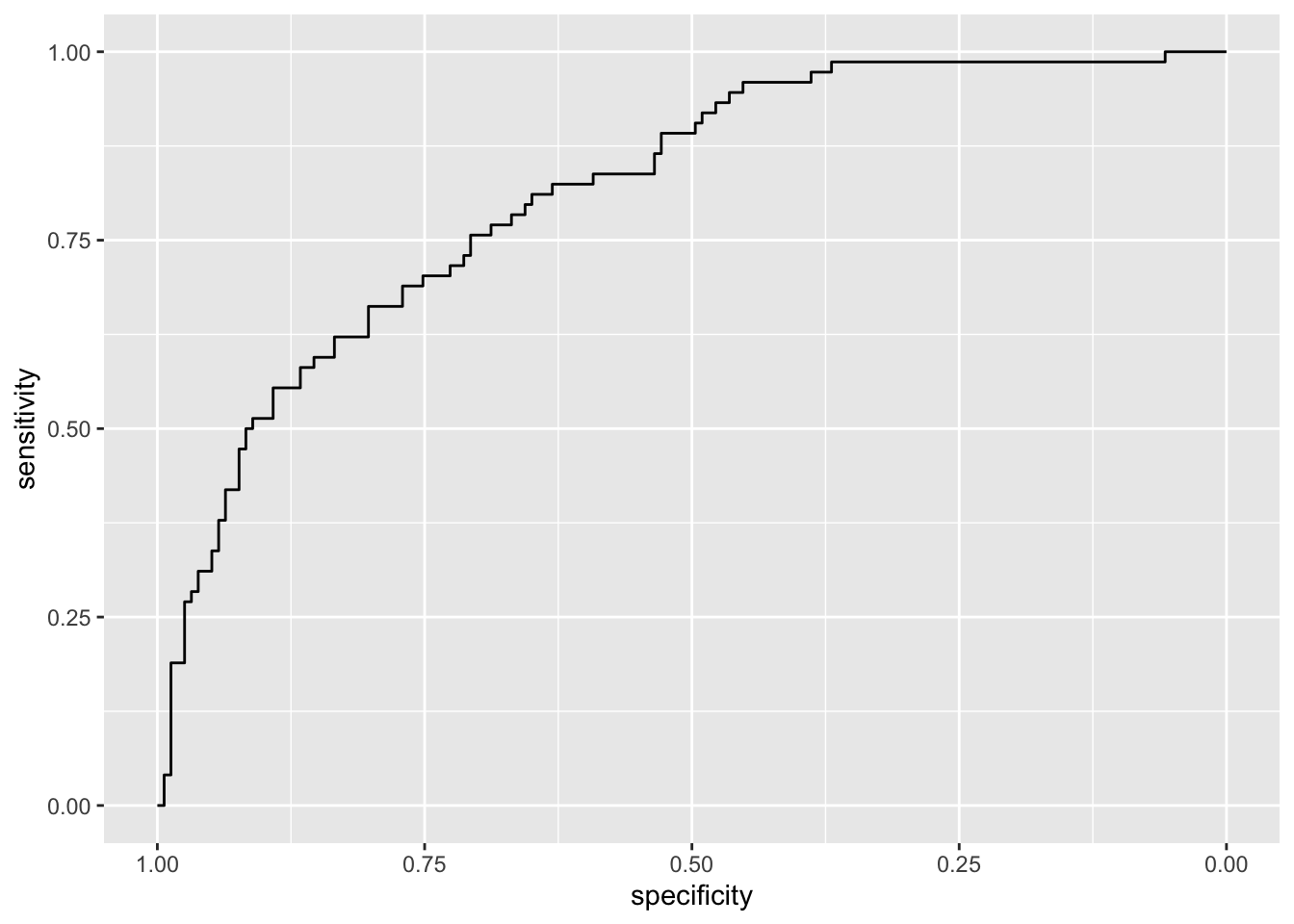 Note that the plot uses specificity on the x-axis (which goes from 1 on the left to zero on the right) and sensitivity on the y-axis.
We now compute all the ROC curves and plot them together using the ggroc function:
roc_lda = roc(d_test$Outcome,
              lda_pred$posterior[,2]) #2nd col with Yes probs
## Setting levels: control = No, case = Yes## Setting direction: controls < casesroc_qda = roc(d_test$Outcome,
qda_pred$posterior[,2]) #2nd col with Yes probs## Setting levels: control = No, case = Yes
## Setting direction: controls < casesroc_nb = roc(d_test$Outcome,
nb_pred_prob[,2])## Setting levels: control = No, case = Yes
## Setting direction: controls < casesggroc(list(logreg = roc_logreg,
lda = roc_lda,
qda = roc_qda,
nb = roc_nb))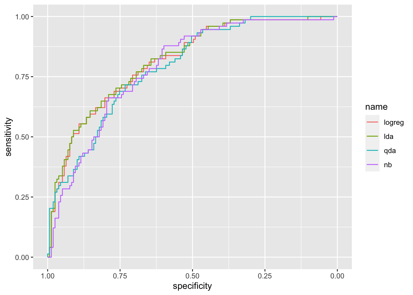
It can be observed that the ROC curve lies below the other two curves meaning that QDA performs worse. Let’s compute the auc for the three methods:
auc(roc_logreg)## Area under the curve: 0.8142auc(roc_lda)## Area under the curve: 0.8186auc(roc_qda)## Area under the curve: 0.7915auc(roc_nb)## Area under the curve: 0.7898LDA shows the highest auc (even if very similar to the other values). All in all we can conclude that LDA is the best classifier.