Chapter 2 R Lab 1 - 24/03/2023
In this lecture we will learn how to implement the K-nearest neighbors (KNN) method for regression problems.
The following packages are required: FNN and tidyverse.
library(FNN)
library(tidyverse)
2.1 KNN for regression problems
For KNN regression we will use data regarding bike sharing (link). The data are stored in the file named bikesharing.csv which is available in the e-learning. The data regard the bike sharing counts aggregated on daily basis.
We start by importing the data. Please, note that in the following code my file path is shown; obviously for your computer it will be different:
bikesharing <- read.csv("./files/bikesharing.csv")glimpse(bikesharing)## Rows: 731
## Columns: 16
## $ instant <int> 1, 2, 3, 4, 5, 6, 7, 8, 9, 10, 11, 12, 13, 14, 15, 16, 17, 18, 19, 2…
## $ dteday <chr> "2011-01-01", "2011-01-02", "2011-01-03", "2011-01-04", "2011-01-05"…
## $ season <int> 1, 1, 1, 1, 1, 1, 1, 1, 1, 1, 1, 1, 1, 1, 1, 1, 1, 1, 1, 1, 1, 1, 1,…
## $ yr <int> 0, 0, 0, 0, 0, 0, 0, 0, 0, 0, 0, 0, 0, 0, 0, 0, 0, 0, 0, 0, 0, 0, 0,…
## $ mnth <int> 1, 1, 1, 1, 1, 1, 1, 1, 1, 1, 1, 1, 1, 1, 1, 1, 1, 1, 1, 1, 1, 1, 1,…
## $ holiday <int> 0, 0, 0, 0, 0, 0, 0, 0, 0, 0, 0, 0, 0, 0, 0, 0, 1, 0, 0, 0, 0, 0, 0,…
## $ weekday <int> 6, 0, 1, 2, 3, 4, 5, 6, 0, 1, 2, 3, 4, 5, 6, 0, 1, 2, 3, 4, 5, 6, 0,…
## $ workingday <int> 0, 0, 1, 1, 1, 1, 1, 0, 0, 1, 1, 1, 1, 1, 0, 0, 0, 1, 1, 1, 1, 0, 0,…
## $ weathersit <int> 2, 2, 1, 1, 1, 1, 2, 2, 1, 1, 2, 1, 1, 1, 2, 1, 2, 2, 2, 2, 1, 1, 1,…
## $ temp <dbl> 0.3441670, 0.3634780, 0.1963640, 0.2000000, 0.2269570, 0.2043480, 0.…
## $ atemp <dbl> 0.3636250, 0.3537390, 0.1894050, 0.2121220, 0.2292700, 0.2332090, 0.…
## $ hum <dbl> 0.805833, 0.696087, 0.437273, 0.590435, 0.436957, 0.518261, 0.498696…
## $ windspeed <dbl> 0.1604460, 0.2485390, 0.2483090, 0.1602960, 0.1869000, 0.0895652, 0.…
## $ casual <int> 331, 131, 120, 108, 82, 88, 148, 68, 54, 41, 43, 25, 38, 54, 222, 25…
## $ registered <int> 654, 670, 1229, 1454, 1518, 1518, 1362, 891, 768, 1280, 1220, 1137, …
## $ cnt <int> 985, 801, 1349, 1562, 1600, 1606, 1510, 959, 822, 1321, 1263, 1162, …The dataset is composed by 731 rows (i.e. days) and 16 variables. We are in particular interested in the following quantitative variables (in this case \(p=3\) regressors):
atemp: normalized feeling temperature in Celsiushum: normalized humiditywindspeed: normalized wind speedcnt: count of total rental bikes (response variable)
The response variable cnt can be summarized as follows:
summary(bikesharing$cnt)## Min. 1st Qu. Median Mean 3rd Qu. Max.
## 22 3152 4548 4504 5956 8714bikesharing %>%
ggplot()+
geom_histogram(aes(cnt),bins=10,col="white")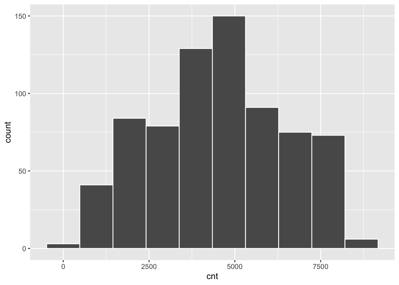
Obviously, the number of bike rentals depends strongly on weather conditions. In the following plot we represent cnt as a function of atemp and windspeed, specifying a scale color from yellow to dark blue with 12 levels:
bikesharing %>%
  ggplot()+
  geom_point(aes(x=atemp,y=windspeed,col=cnt))+
  scale_colour_gradient(low="blue", high="red")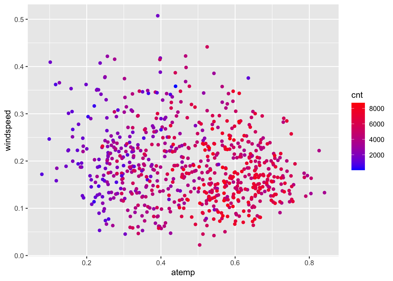
It can be observed that the number of bike rentals increases with temperature.
2.2 Creation of the training and testing set: method 1
We divide the dataset into 3 subsets:
- training set: containing 70% of the observations
- validating set: containing 15% of the observations
- test set: containing 15% of the observations
The procedure is done randomly by using the function sample. In order to have reproducible results, it is necessary to set the seed. We create the vector index, that will be later added to bikesharing. This index vector contains for each observation a value (that can be 1, 2 or 3) defining the group where the observation will be included (training, validation or test).
set.seed(55)
# Sample the indexes for the training observations
index <- sample(1:3,
                size = nrow(bikesharing),
                prob = c(0.7,0.15,0.15),
                replace=T) # the same value from (1,2 or 3) can be sampled more than once!

head(index)
## [1] 1 1 1 3 1 1bikesharing$index = index
glimpse(bikesharing)## Rows: 731
## Columns: 17
## $ instant <int> 1, 2, 3, 4, 5, 6, 7, 8, 9, 10, 11, 12, 13, 14, 15, 16, 17, 18, 19, 2…
## $ dteday <chr> "2011-01-01", "2011-01-02", "2011-01-03", "2011-01-04", "2011-01-05"…
## $ season <int> 1, 1, 1, 1, 1, 1, 1, 1, 1, 1, 1, 1, 1, 1, 1, 1, 1, 1, 1, 1, 1, 1, 1,…
## $ yr <int> 0, 0, 0, 0, 0, 0, 0, 0, 0, 0, 0, 0, 0, 0, 0, 0, 0, 0, 0, 0, 0, 0, 0,…
## $ mnth <int> 1, 1, 1, 1, 1, 1, 1, 1, 1, 1, 1, 1, 1, 1, 1, 1, 1, 1, 1, 1, 1, 1, 1,…
## $ holiday <int> 0, 0, 0, 0, 0, 0, 0, 0, 0, 0, 0, 0, 0, 0, 0, 0, 1, 0, 0, 0, 0, 0, 0,…
## $ weekday <int> 6, 0, 1, 2, 3, 4, 5, 6, 0, 1, 2, 3, 4, 5, 6, 0, 1, 2, 3, 4, 5, 6, 0,…
## $ workingday <int> 0, 0, 1, 1, 1, 1, 1, 0, 0, 1, 1, 1, 1, 1, 0, 0, 0, 1, 1, 1, 1, 0, 0,…
## $ weathersit <int> 2, 2, 1, 1, 1, 1, 2, 2, 1, 1, 2, 1, 1, 1, 2, 1, 2, 2, 2, 2, 1, 1, 1,…
## $ temp <dbl> 0.3441670, 0.3634780, 0.1963640, 0.2000000, 0.2269570, 0.2043480, 0.…
## $ atemp <dbl> 0.3636250, 0.3537390, 0.1894050, 0.2121220, 0.2292700, 0.2332090, 0.…
## $ hum <dbl> 0.805833, 0.696087, 0.437273, 0.590435, 0.436957, 0.518261, 0.498696…
## $ windspeed <dbl> 0.1604460, 0.2485390, 0.2483090, 0.1602960, 0.1869000, 0.0895652, 0.…
## $ casual <int> 331, 131, 120, 108, 82, 88, 148, 68, 54, 41, 43, 25, 38, 54, 222, 25…
## $ registered <int> 654, 670, 1229, 1454, 1518, 1518, 1362, 891, 768, 1280, 1220, 1137, …
## $ cnt <int> 985, 801, 1349, 1562, 1600, 1606, 1510, 959, 822, 1321, 1263, 1162, …
## $ index <int> 1, 1, 1, 3, 1, 1, 1, 1, 1, 1, 2, 1, 1, 1, 1, 3, 1, 2, 1, 1, 1, 3, 1,…We now create three different datasets filtering by index:
bikesharing_tr = bikesharing %>%
  filter(index == 1)

bikesharing_val = bikesharing %>%
  filter(index == 2)

bikesharing_te = bikesharing %>%
  filter(index == 3)
The validation set will be used to tune the model, i.e. to choose the best value of the tuning parameter (the number of neighbors) which minimizes the validation error. Finally, we will rejoin together training and validation datasets and we will calculate the final Test MSE (to be later compared with other models).
2.2.1 Implementation of KNN regression with \(K=1\)
The function used to implement KNN regression is knn.reg from the FNN package (see ?knn.reg). We start by considering the case when \(K=1\), corresponding to the most flexible model, when only one neighbor is considered.
In the argument train and test of the knn.reg function it is necessary to provide the 3 regressors from the training and validation dataset. In this case we select directly the necessary variables from the existing dataframes (bikesharing_tr and bikesharing_val) by using the function select from the dplyr package (part of tidyverse collection). Finally, the arguments y and k refer to the training response variable vector and the number of neighbors, respectively.
KNN1 = knn.reg(train = dplyr::select(bikesharing_tr,atemp,windspeed,hum),
                   test = dplyr::select(bikesharing_val,atemp,windspeed,hum),
                   y = dplyr::select(bikesharing_tr, cnt),
                   k = 1)
The object KNN1 contains different objects
names(KNN1)## [1] "call" "k" "n" "pred" "residuals" "PRESS" "R2Pred"We are in particular interested in the object pred which contains the predictions \(\hat y_0\) for the test observations. It is then possible to compute the test mean square error (MSE):
\[
\text{mean}(y_0-\hat y_0)^2
\]
where average is computed over all the observations in the validation set.
# Compute the validation MSE for K=1
mean((bikesharing_val$cnt - KNN1$pred)^2)
## [1] 2817811It is also possible to plot observed and predicted values. To do this we first create a new dataframe containing the observed values (\(y_0\)) and the KNN predictions (\(\hat y_0\)). Then we represent graphically the observed and predicted values and assign to the points a color given by the values of the squared error:
data.frame(obs=bikesharing_val$cnt,
pred=KNN1$pred) %>%
ggplot() +
geom_point(aes(x=obs,y=pred,col=(obs-pred)^2)) +
scale_color_gradient(low="blue",high="red")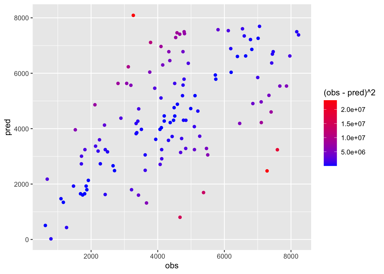 Blue observations are characterized by a smaller squared error meaning that predictions are close to observed values.
2.2.2 Implementation of KNN regression with different values of \(K\)
We now use a for loop to implement automatically the KNN regression for different values of \(K\) . In particular, we consider the values 1, 10, 25,100, 200, 500. Each step of the loop, indexed by a variable i, considers a different value of \(K\). We want to save in a vector all the values of the test MSE.
# Create an empty vector where values of the MSE will be saved
mse_vec = c()
# Create a vector with the values of k
k_vec = c(1, 10, 25, 100, 200, 500)
# Start the for loop
for(i in 1:length(k_vec)){

  # Run KNN
  KNN = knn.reg(train = dplyr::select(bikesharing_tr,atemp, windspeed,hum),
                     test = dplyr::select(bikesharing_val,atemp, windspeed,hum),
                     y = dplyr::select(bikesharing_tr, cnt),
                     k = k_vec[i])
  # Save the MSE
  mse_vec[i] = mean((bikesharing_val$cnt-KNN$pred)^2)

}
The value of the test MSE are the following:
mse_vec## [1] 2817811 1596671 1668400 1814851 2100513 3567147It is useful to plot the values of the test MSE as a function of \(K\):
data.frame(k_vec, mse_vec) %>%
  ggplot() +
  geom_line(aes(k_vec,mse_vec)) +
  geom_point(aes(k_vec,mse_vec))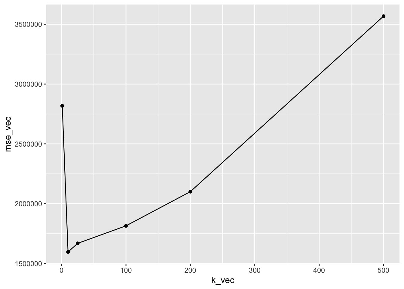
We want now to save the value of \(K\) which minimizes the MSE:
kbest = data.frame(k_vec, mse_vec) %>%
  filter(mse_vec == min(mse_vec)) %>%
  dplyr::select(k_vec) %>%
  pull()
kbest
## [1] 10The function pull is used to transform a data frame into a vector (in this case the best value of \(K\) which is a scalar).
2.2.3 Assessment of the tuned model
Now we can finally calculate the Test MSE with the selected parameter. Now that tuning is over we join together the training and the validation data using bind_rows:
bikesharing_newtr = bind_rows(bikesharing_val, bikesharing_tr)
dim(bikesharing_newtr)
## [1] 633 17Then we run KNN with the best value of \(K\) kbest and the new training data bikesharing_newtr:
KNNbest <- knn.reg(train = dplyr::select(bikesharing_newtr, atemp, hum, windspeed),
                test = dplyr::select(bikesharing_te, atemp, hum, windspeed),
                y = dplyr::select(bikesharing_newtr,cnt),
                k=kbest)

MSE_KNN_final = mean((bikesharing_te$cnt - KNNbest$pred)^2)
MSE_KNN_final
## [1] 14992622.2.4 Comparison of KNN with the multiple linear model
We consider for the same set of data also the multiple linear model with 3 regressors: \[ Y = \beta_0+\beta_1 X_1+\beta_2 X_2+\beta_3 X_3 +\epsilon \]
This can be implemented by using the lm function applied to the training set of data:
modlm = lm(cnt ~ atemp+windspeed+hum,
           data = bikesharing_newtr)
summary(modlm)
##
## Call:
## lm(formula = cnt ~ atemp + windspeed + hum, data = bikesharing_newtr)
##
## Residuals:
## Min 1Q Median 3Q Max
## -4922.4 -1039.6 -85.9 1062.1 4361.9
##
## Coefficients:
## Estimate Std. Error t value Pr(>|t|)
## (Intercept) 3779.8 366.6 10.31 < 2e-16 ***
## atemp 7506.8 357.6 20.99 < 2e-16 ***
## windspeed -4313.4 752.8 -5.73 1.56e-08 ***
## hum -3180.3 415.2 -7.66 7.03e-14 ***
## ---
## Signif. codes: 0 '***' 0.001 '**' 0.01 '*' 0.05 '.' 0.1 ' ' 1
##
## Residual standard error: 1427 on 629 degrees of freedom
## Multiple R-squared: 0.4593, Adjusted R-squared: 0.4568
## F-statistic: 178.1 on 3 and 629 DF, p-value: < 2.2e-16The corresponding predictions and test MSE can be obtained as follows by making use of the predict function:
predlm = predict(modlm,
                 newdata = bikesharing_te)
MSE_lm = mean((bikesharing_te$cnt-predlm)^2)
MSE_lm
## [1] 1933325Note that the test MSE of the linear regression model is higher than the KNN MSE.
2.2.5 Comparison of KNN with the multiple linear model with quadratic terms
For introducing some flexibility we try to extend the previous linear model by including quadratic terms of the regressors: \[ Y = \beta_0+\beta_1 X_1+\beta_2 X_2+\beta_3 X_3 + \beta_4 X_1^2 + \beta_5 X_2^2 + \beta_6 X_3^2+\epsilon \]
This is still a linear model in the parameters (not in the variables). Polynomial regression models are able to produce non-linear fitted functions.
This model can be implemented by using the poly function (with degree=2 in this case) in the formula specification. This specifies a model including \(X\) and \(X^2\).
modlmpoly = lm(cnt ~ poly(atemp,2) +
                 poly(windspeed,2)+
                 poly(hum,2), data=bikesharing_newtr)
summary(modlmpoly)
##
## Call:
## lm(formula = cnt ~ poly(atemp, 2) + poly(windspeed, 2) + poly(hum,
## 2), data = bikesharing_newtr)
##
## Residuals:
## Min 1Q Median 3Q Max
## -3271.7 -959.1 -120.3 1074.2 4545.9
##
## Coefficients:
## Estimate Std. Error t value Pr(>|t|)
## (Intercept) 4499.38 50.88 88.429 < 2e-16 ***
## poly(atemp, 2)1 30111.90 1319.85 22.815 < 2e-16 ***
## poly(atemp, 2)2 -14865.73 1329.55 -11.181 < 2e-16 ***
## poly(windspeed, 2)1 -7422.92 1361.56 -5.452 7.18e-08 ***
## poly(windspeed, 2)2 201.07 1292.41 0.156 0.876
## poly(hum, 2)1 -14501.19 1366.54 -10.612 < 2e-16 ***
## poly(hum, 2)2 -8767.96 1330.21 -6.591 9.26e-11 ***
## ---
## Signif. codes: 0 '***' 0.001 '**' 0.01 '*' 0.05 '.' 0.1 ' ' 1
##
## Residual standard error: 1280 on 626 degrees of freedom
## Multiple R-squared: 0.5672, Adjusted R-squared: 0.563
## F-statistic: 136.7 on 6 and 626 DF, p-value: < 2.2e-16As before we compute the test MSE:
predlmpoly = predict(modlmpoly,
                  newdata = bikesharing_te)
MSE_lm2 = mean((bikesharing_te$cnt-predlmpoly)^2)
MSE_lm2
## [1] 15180432.2.6 Final comparison
We can now compare the MSE of the best KNN model and of the 2 linear regression models:
MSE_KNN_final## [1] 1499262MSE_lm## [1] 1933325MSE_lm2## [1] 1518043Results show that the multiple linear regression model has the worst performance. The polynomial model and the KNN have a similar performance.