Chapter 3 R Lab 2 - 04/04/2023
In this lecture we will learn how to implement KNN and the linear discriminant analysis (LDA) for a classification problem. Moreover, the methods will be compared by using performance indexes.
The following packages are required: class, MASS and tidyverse.
library(MASS) #for LDA
library(tidyverse)
library(class) #for KNN classification
3.1 Loan default data
The data we use for this lab are taken from the book titled “Machine Learning & Data Science Blueprints for Finance” (suggested for the AIMLFF course). See in particular the Case Study 2: loan default probability in Chapter 6. The goal is to build machine learning models to predict the probability that a loan will default and won’t be repaid by the borrower.
The response variable is named charged_off and is a binary integer variable: 0 means that the borrower was able to fully pay the loan, while 1 means that the loan was charged off (default). In this case study there are several regressors, both quantitative and qualitative.
We import the data as usual
d <- read.csv("./files/loandefault.csv")
glimpse(d)
## Rows: 86,138
## Columns: 34
## $ loan_amnt <dbl> 15000, 10400, 21425, 7650, 9600, 2500, 16000, 23325, 5250…
## $ funded_amnt <dbl> 15000, 10400, 21425, 7650, 9600, 2500, 16000, 23325, 5250…
## $ term <chr> " 60 months", " 36 months", " 60 months", " 36 months", "…
## $ int_rate <dbl> 12.39, 6.99, 15.59, 13.66, 13.66, 11.99, 11.44, 14.31, 11…
## $ installment <dbl> 336.64, 321.08, 516.36, 260.20, 326.53, 83.03, 351.40, 80…
## $ grade <chr> "C", "A", "D", "C", "C", "B", "B", "C", "B", "B", "D", "C…
## $ sub_grade <chr> "C1", "A3", "D1", "C3", "C3", "B5", "B4", "C4", "B4", "B5…
## $ emp_title <chr> "MANAGEMENT", "Truck Driver Delivery Personel", "Programm…
## $ emp_length <chr> "10+ years", "8 years", "6 years", "< 1 year", "10+ years…
## $ home_ownership <chr> "RENT", "MORTGAGE", "RENT", "RENT", "RENT", "MORTGAGE", "…
## $ annual_inc <dbl> 78000, 58000, 63800, 50000, 69000, 89000, 109777, 72000, …
## $ verification_status <chr> "Source Verified", "Not Verified", "Source Verified", "So…
## $ purpose <chr> "debt_consolidation", "credit_card", "credit_card", "debt…
## $ title <chr> "Debt consolidation", "Credit card refinancing", "Credit …
## $ zip_code <chr> "235xx", "937xx", "658xx", "850xx", "077xx", "554xx", "20…
## $ addr_state <chr> "VA", "CA", "MO", "AZ", "NJ", "MN", "VA", "WA", "MD", "MI…
## $ dti <dbl> 12.03, 14.92, 18.49, 34.81, 25.81, 13.77, 11.63, 27.03, 1…
## $ earliest_cr_line <chr> "Aug-1994", "Sep-1989", "Aug-2003", "Aug-2002", "Nov-1992…
## $ fico_range_low <dbl> 750, 710, 685, 685, 680, 685, 700, 665, 745, 675, 680, 67…
## $ fico_range_high <dbl> 754, 714, 689, 689, 684, 689, 704, 669, 749, 679, 684, 67…
## $ open_acc <dbl> 6, 17, 10, 11, 12, 9, 7, 14, 8, 5, 11, 7, 11, 10, 7, 9, 3…
## $ revol_util <dbl> 29.0, 31.6, 76.2, 91.9, 59.4, 94.3, 60.4, 82.2, 20.2, 98.…
## $ initial_list_status <chr> "w", "w", "w", "f", "f", "f", "w", "f", "f", "f", "f", "f…
## $ last_pymnt_amnt <dbl> 12017.81, 321.08, 17813.19, 17.70, 9338.58, 2294.26, 4935…
## $ application_type <chr> "Individual", "Individual", "Individual", "Individual", "…
## $ acc_open_past_24mths <dbl> 5, 7, 4, 6, 8, 6, 3, 6, 4, 0, 7, 2, 5, 6, 2, 6, 3, 4, 6, …
## $ avg_cur_bal <dbl> 29828, 9536, 4232, 5857, 3214, 44136, 53392, 39356, 1267,…
## $ bc_open_to_buy <dbl> 9525, 7599, 324, 332, 6494, 1333, 2559, 3977, 12152, 324,…
## $ bc_util <dbl> 4.7, 41.5, 97.8, 93.2, 69.2, 86.4, 72.2, 89.0, 26.8, 98.5…
## $ mo_sin_old_rev_tl_op <dbl> 244, 290, 136, 148, 265, 148, 133, 194, 67, 124, 122, 167…
## $ mo_sin_rcnt_rev_tl_op <dbl> 1, 1, 7, 8, 23, 24, 17, 15, 12, 40, 2, 21, 15, 8, 27, 3, …
## $ mort_acc <dbl> 0, 1, 0, 0, 0, 5, 2, 6, 0, 0, 0, 2, 5, 0, 0, 0, 0, 1, 0, …
## $ num_actv_rev_tl <dbl> 4, 9, 4, 4, 7, 4, 3, 5, 2, 5, 8, 3, 8, 6, 3, 2, 2, 5, 6, …
## $ charged_off <int> 0, 1, 0, 1, 0, 0, 0, 1, 0, 1, 1, 0, 0, 0, 0, 0, 0, 0, 0, …3.2 Data preparation and cleaning
The following steps follows the approach used in the book. As we will implement LDA and KNN, we need to have only quantitative regressors (is.numeric). They can be jointly selected by using the function select_if (we create a new data frame called data2):
d2 = d %>% select_if(is.numeric)
glimpse(d2)
## Rows: 86,138
## Columns: 20
## $ loan_amnt <dbl> 15000, 10400, 21425, 7650, 9600, 2500, 16000, 23325, 5250…
## $ funded_amnt <dbl> 15000, 10400, 21425, 7650, 9600, 2500, 16000, 23325, 5250…
## $ int_rate <dbl> 12.39, 6.99, 15.59, 13.66, 13.66, 11.99, 11.44, 14.31, 11…
## $ installment <dbl> 336.64, 321.08, 516.36, 260.20, 326.53, 83.03, 351.40, 80…
## $ annual_inc <dbl> 78000, 58000, 63800, 50000, 69000, 89000, 109777, 72000, …
## $ dti <dbl> 12.03, 14.92, 18.49, 34.81, 25.81, 13.77, 11.63, 27.03, 1…
## $ fico_range_low <dbl> 750, 710, 685, 685, 680, 685, 700, 665, 745, 675, 680, 67…
## $ fico_range_high <dbl> 754, 714, 689, 689, 684, 689, 704, 669, 749, 679, 684, 67…
## $ open_acc <dbl> 6, 17, 10, 11, 12, 9, 7, 14, 8, 5, 11, 7, 11, 10, 7, 9, 3…
## $ revol_util <dbl> 29.0, 31.6, 76.2, 91.9, 59.4, 94.3, 60.4, 82.2, 20.2, 98.…
## $ last_pymnt_amnt <dbl> 12017.81, 321.08, 17813.19, 17.70, 9338.58, 2294.26, 4935…
## $ acc_open_past_24mths <dbl> 5, 7, 4, 6, 8, 6, 3, 6, 4, 0, 7, 2, 5, 6, 2, 6, 3, 4, 6, …
## $ avg_cur_bal <dbl> 29828, 9536, 4232, 5857, 3214, 44136, 53392, 39356, 1267,…
## $ bc_open_to_buy <dbl> 9525, 7599, 324, 332, 6494, 1333, 2559, 3977, 12152, 324,…
## $ bc_util <dbl> 4.7, 41.5, 97.8, 93.2, 69.2, 86.4, 72.2, 89.0, 26.8, 98.5…
## $ mo_sin_old_rev_tl_op <dbl> 244, 290, 136, 148, 265, 148, 133, 194, 67, 124, 122, 167…
## $ mo_sin_rcnt_rev_tl_op <dbl> 1, 1, 7, 8, 23, 24, 17, 15, 12, 40, 2, 21, 15, 8, 27, 3, …
## $ mort_acc <dbl> 0, 1, 0, 0, 0, 5, 2, 6, 0, 0, 0, 2, 5, 0, 0, 0, 0, 1, 0, …
## $ num_actv_rev_tl <dbl> 4, 9, 4, 4, 7, 4, 3, 5, 2, 5, 8, 3, 8, 6, 3, 2, 2, 5, 6, …
## $ charged_off <int> 0, 1, 0, 1, 0, 0, 0, 1, 0, 1, 1, 0, 0, 0, 0, 0, 0, 0, 0, …The next step is to transform the response variable (now coded as 0/1 integer variable) into a factor (qualitative variable) with categories 0_FullyPaid and 1_ChargedOff. Note that we check the frequency distribution of the variable charged_off before and after the transformation to be sure that everything works fine:
d2 %>% count(charged_off)## charged_off n
## 1 0 69982
## 2 1 16156# from integer to factor
d2$charged_off = factor(d2$charged_off,
levels = c(0,1),
labels = c("0_FullyPaid", "1_ChargedOff"))
d2 %>% count(charged_off)## charged_off n
## 1 0_FullyPaid 69982
## 2 1_ChargedOff 16156We can now plot the frequency distribution for charged_off as follows using the geom_bar geometry (automatically in the y-axis absolute frequencies - count - are reported):
d2 %>%
  ggplot()+
  geom_bar(aes(charged_off), fill="pink")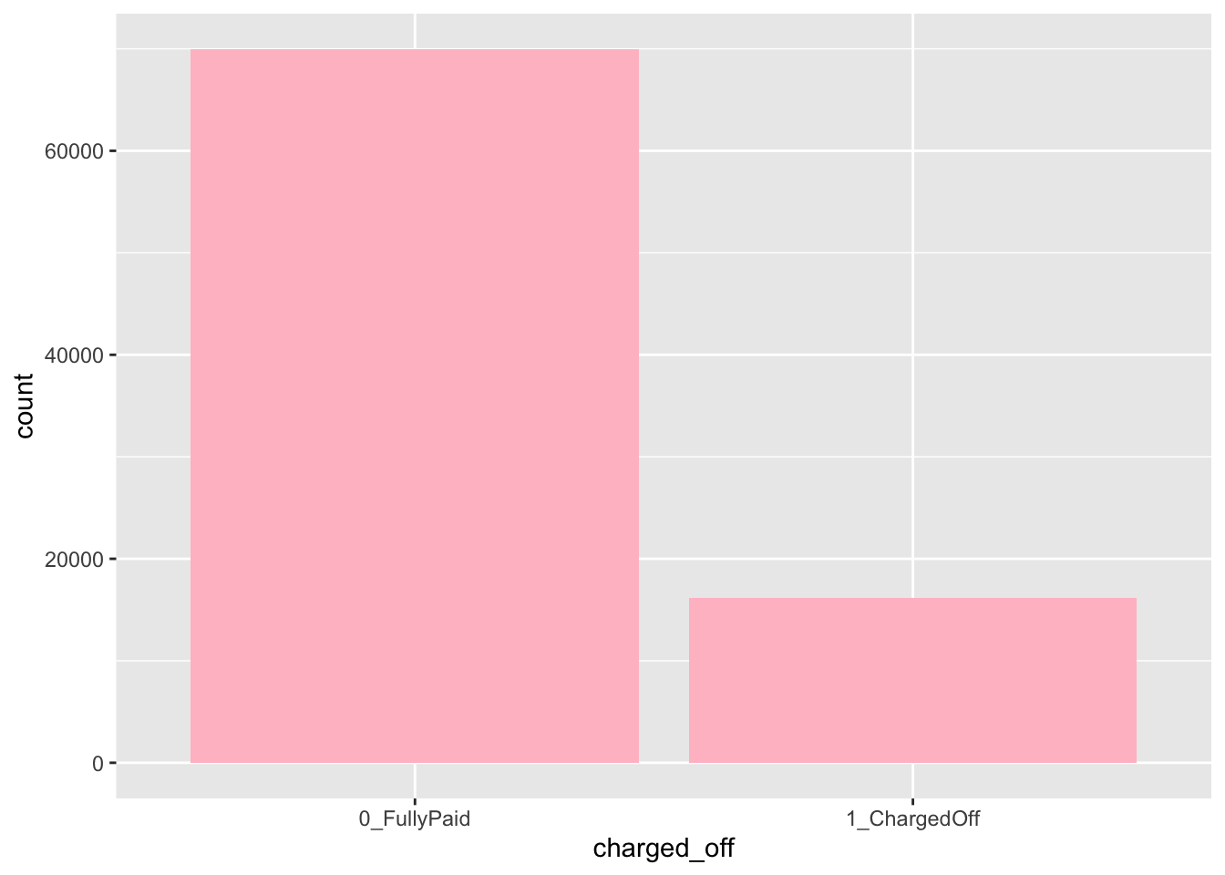
If we run the summary function we realize that some of the variables have missing values (e.g. bc_open_to_buy):
summary(d2)## loan_amnt funded_amnt int_rate installment annual_inc
## Min. : 1000 Min. : 1000 Min. : 6.00 Min. : 30.42 Min. : 4000
## 1st Qu.: 7800 1st Qu.: 7800 1st Qu.: 9.49 1st Qu.: 248.48 1st Qu.: 45000
## Median :12000 Median :12000 Median :12.99 Median : 370.48 Median : 62474
## Mean :14107 Mean :14107 Mean :13.00 Mean : 430.74 Mean : 73843
## 3rd Qu.:20000 3rd Qu.:20000 3rd Qu.:15.61 3rd Qu.: 568.00 3rd Qu.: 90000
## Max. :35000 Max. :35000 Max. :26.06 Max. :1408.13 Max. :7500000
##
## dti fico_range_low fico_range_high open_acc revol_util
## Min. : 0.00 Min. :660.0 Min. :664.0 Min. : 1.00 Min. : 0.00
## 1st Qu.:12.07 1st Qu.:670.0 1st Qu.:674.0 1st Qu.: 8.00 1st Qu.: 37.20
## Median :17.95 Median :685.0 Median :689.0 Median :11.00 Median : 54.90
## Mean :18.53 Mean :692.5 Mean :696.5 Mean :11.75 Mean : 54.58
## 3rd Qu.:24.50 3rd Qu.:705.0 3rd Qu.:709.0 3rd Qu.:14.00 3rd Qu.: 72.50
## Max. :39.99 Max. :845.0 Max. :850.0 Max. :84.00 Max. :180.30
## NA's :44
## last_pymnt_amnt acc_open_past_24mths avg_cur_bal bc_open_to_buy
## Min. : 0.0 Min. : 0.000 Min. : 0 Min. : 0
## 1st Qu.: 358.5 1st Qu.: 2.000 1st Qu.: 3010 1st Qu.: 1087
## Median : 1241.2 Median : 4.000 Median : 6994 Median : 3823
## Mean : 4757.4 Mean : 4.595 Mean : 13067 Mean : 8943
## 3rd Qu.: 7303.2 3rd Qu.: 6.000 3rd Qu.: 17905 3rd Qu.: 10588
## Max. :36234.4 Max. :53.000 Max. :447433 Max. :249625
## NA's :996
## bc_util mo_sin_old_rev_tl_op mo_sin_rcnt_rev_tl_op mort_acc
## Min. : 0.00 Min. : 3.0 Min. : 0.0 Min. : 0.000
## 1st Qu.: 44.10 1st Qu.:118.0 1st Qu.: 3.0 1st Qu.: 0.000
## Median : 67.70 Median :167.0 Median : 8.0 Median : 1.000
## Mean : 63.81 Mean :183.5 Mean : 12.8 Mean : 1.749
## 3rd Qu.: 87.50 3rd Qu.:232.0 3rd Qu.: 15.0 3rd Qu.: 3.000
## Max. :255.20 Max. :718.0 Max. :372.0 Max. :34.000
## NA's :1049
## num_actv_rev_tl charged_off
## Min. : 0.000 0_FullyPaid :69982
## 1st Qu.: 3.000 1_ChargedOff:16156
## Median : 5.000
## Mean : 5.762
## 3rd Qu.: 7.000
## Max. :38.000
## One possibility is to do data imputation for the missing values. Here instead we will remove the observations (rows) with one or more than one missing values by using na.omit:
d2 = na.omit(d2)Note the reduction in the number of observation for d2 after removing the missing values.
From the preview of the data and the summary statistics we realize that loan_amnt and funded_amnt have the same values. To be sure that these two variables take exactly the same values we plot them joint using a scatterplot:
d2 %>%
  ggplot()+
  geom_point(aes(funded_amnt,loan_amnt))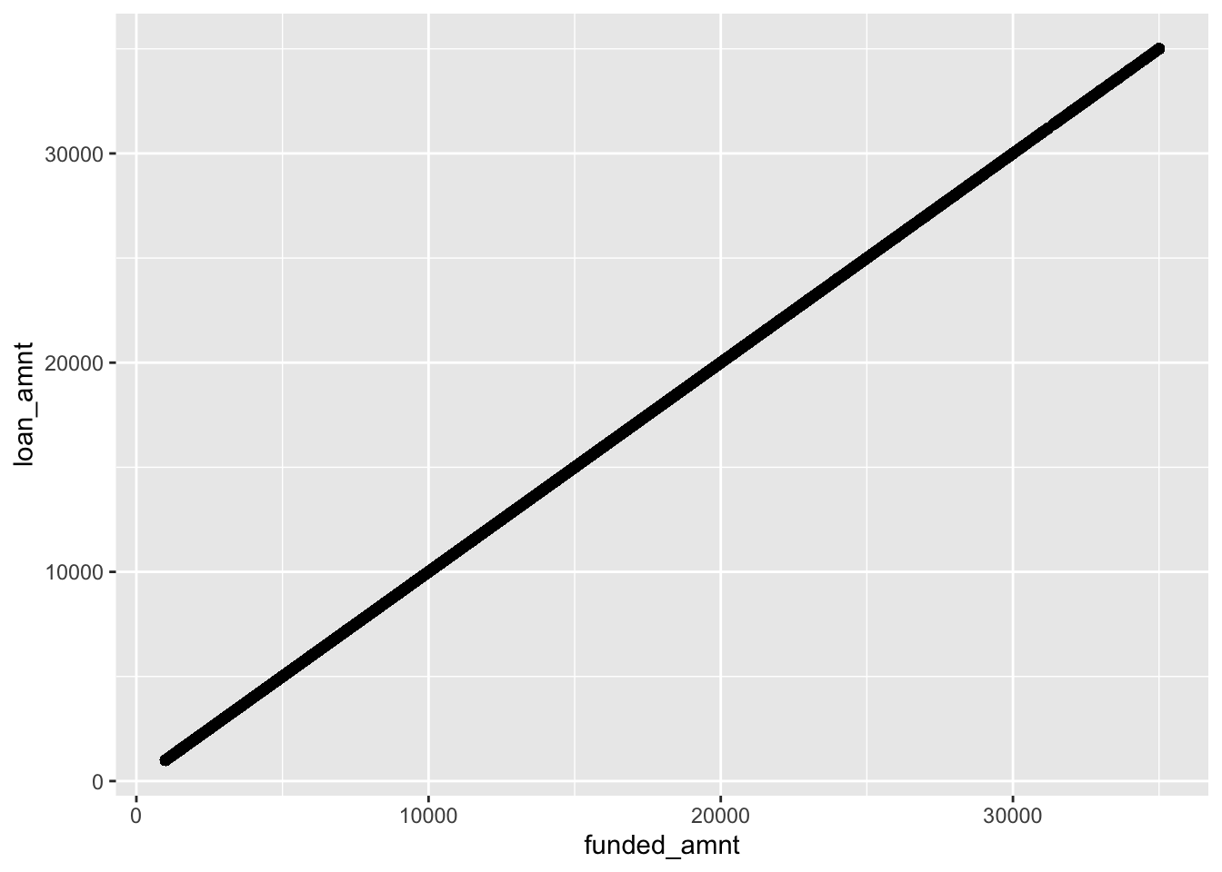
As the points are exactly on a straight line it means that they exactly coincide. Thus, we need to remove one of the two for avoiding problems with the models’ estimation:
# Remove funded_amnt
d2 = d2 %>% dplyr::select(- funded_amnt)
Note that the code dplyr::select here above is used to specify that the function select is from the dplyr package (which is part of the tidyverse collection). This is required because sometimes select gives some weird error…
We then plot the distribution of annual_inc conditionally on charged_off by using boxplots:
d2 %>%
  ggplot()+
  geom_boxplot(aes(charged_off, annual_inc))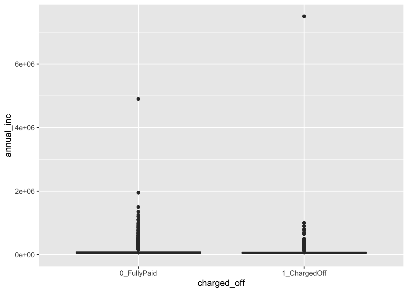
We see that, due to the extreme values in the annual_inc the boxes are completely hidden and the distribution of the variable is not clearly shown. We try to apply the log transformation to the quantitative variable:
d2 %>%
  ggplot()+
  geom_boxplot(aes(charged_off,  log(annual_inc)))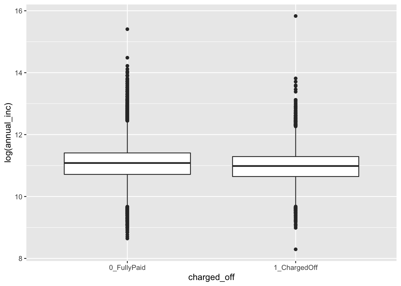
Now, the distribuion appears more reasonable for both the categories (the median annual_inc is very similar in the two groups). We thus decide to apply this transformation permanently in the dataframe by creating a new variable named log_annual_inc and eliminating the old one:
d2 = d2 %>%
  mutate(log_annual_inc = log(annual_inc)) %>%
  dplyr::select(-annual_inc) #remove the original income
We check now the correlation between the fico_range_high and fico_range_low, where the FICO score is designed to rank-order consumers by their sensitivity to a future economic downturn.
cor(d2$fico_range_high, d2$fico_range_low)## [1] 1The correlation is exactly equal to one meaning that the two variables are perfectly linearly associated, see also the following plot:
d2 %>%
  ggplot()+
  geom_point(aes(fico_range_high, fico_range_low))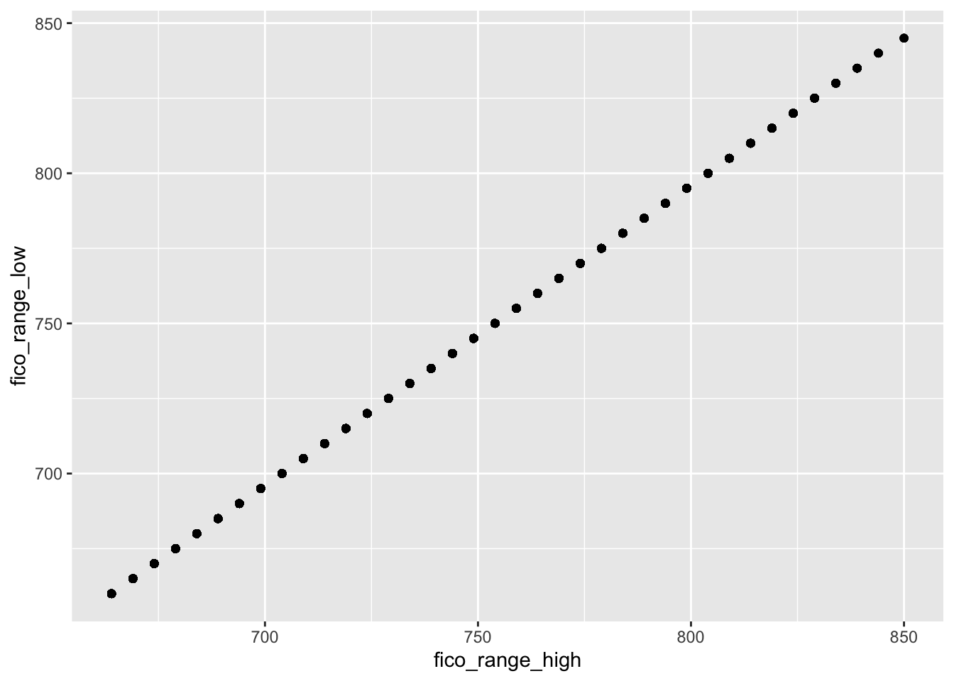
This means that it doesn’t make sense to have both the variables for the modeling because they provide the same information. We thus create a new variable which is the average of the two (remember to remove the original variables after the creation of fico_new):
d2 = d2 %>%
  mutate(fico_new = (fico_range_high+fico_range_low)/2) %>%
  dplyr::select(-fico_range_high, -fico_range_low)
3.3 A new method for creating the training and testing set
To create the training (80%) and test (20%) dataset we use a new approach different from the one introduced in Section 2.2.
We first create a vector with the indexes we will use for the training dataset. These indexes are sampled randomly in the set of integer between 1 and 85089. In this case we must set replace to FALSE, since each index (corresponding to an observation) can’t be sampled twice since each subject will belong to the training or test set only (not to both). Recall also to set a seed, in order to be able to replicate your results:
set.seed(11)
training_index = sample(1:nrow(d2), nrow(d2)*0.8, replace=F)
head(training_index)
## [1] 65570 66457 19004 73612 28886 37598# positions of the first 6 elements to be included in the training setWe are now ready to sample from the d2 dataset 80% of the observations (rows) by using the training_index vector, and leave the non-sampled indexes for test. Just use a minus (-) before the row selection to exclude them:
# recall: dataset [ row , columns ]
s_train = d2[training_index,]
s_test = d2[-training_index,]
Note that this procedure could be the easiest choice when we don’t have a third dataset (validation).
We are now ready to train our models.
3.4 Definition of a function for computing performance indexes
For assessing the performance of a classifier we compare predicted categories with observed categories. This can be done by using the confusion matrix which is a 2x2 matrix reporting the joint distribution (with absolute frequencies) of predicted (by row) and observed (by column) categories.
| No (obs.) | Yes (obs.) | |||
|---|---|---|---|---|
| No (pred.) | TN | FN | ||
| Yes (pred.) | FP | TP | ||
| Total | N | P |
We consider in particular the following performance indexes:
- sensitivity (true positive rate): TP/P
- specificity (true negative rate): TN/N
- accuracy (rate of correctly classified observations): (TN+TP)/(N+P)
We define a function named perf_indexes which computes the above defined indexes. The function has only one argument which is a confusion 2x2 matrix named cm. It returns a vector with the 3 indexes (sensitivity, specificity, overall accuracy).
perf_indexes = function(cm){
  # True negative rate
  specificity = cm[1,1] / (cm[1,1] + cm[2,1])
  # True positive rate
  sensitivity = cm[2,2] / (cm[1,2] + cm[2,2])
  # Overall accuracy
  accuracy = sum(diag(cm)) / sum(cm)
  # Return all the indexes
  return(c(spec=specificity, sens=sensitivity, acc=accuracy))
}
3.5 KNN for classification problems
For this particular case we assume that the KNN has already been tuned and that the best value for the hyperparameter is \(K=200\). Rememember that usually tuning is necessary, as described in the previous lab with KNN regression.
We now implement KNN classification with \(K=200\) by using the knn function from the class package (see ?knn). Note that there are two functions both named knn in the class and FNN package. In order to specify that we want to use the function in the class package we could use class::knn. We have to specify the regressor dataframe for the training and test observations and the response variable vector (cl).
outknn = knn(train = dplyr::select(s_train, -charged_off),
             test = dplyr::select(s_test, -charged_off),
             cl = s_train$charged_off,
             k = 200)
length(outknn)
## [1] 17018head(outknn)## [1] 0_FullyPaid 0_FullyPaid 0_FullyPaid 0_FullyPaid 0_FullyPaid 0_FullyPaid
## Levels: 0_FullyPaid 1_ChargedOffPredictions (categories) are contained in the outknn object. To compare predictions \(\hat y_0\) and observed values \(y_0\), it is useful to create the confusion matrix which is a double-entry matrix with predicted and observed categories and the corresponding frequencies:
table(pred=outknn, obs=s_test$charged_off)## obs
## pred 0_FullyPaid 1_ChargedOff
## 0_FullyPaid 13199 2291
## 1_ChargedOff 712 816In the main diagonal we can read the number of correctly classified observations. Outside from the main diagonal we have the number of missclassified observations.
The percentage test error rate is computed as follows:
#test error rate
mean(outknn != s_test$charged_off)*100
## [1] 17.64602We also create the function perf_indexes defined above the compute the performance indexes for KNN:
perf_indexes(table(pred=outknn, obs=s_test$charged_off))## spec sens acc
## 0.9488175 0.2626328 0.8235398In this case we see that 82.35% of the observations are correctly classified. However the sensitivity is quite small and we are not able to classify risky individuals (we predict 2291 subjects are 0_FullyPaid but actually they charged off).
3.6 Linear discriminant analysis (LDA)
To run LDA we use the lda function of the MASS package. We have to specify the formula and the data:
outlda = lda(charged_off ~ ., data = s_train)
outlda
## Call:
## lda(charged_off ~ ., data = s_train)
##
## Prior probabilities of groups:
## 0_FullyPaid 1_ChargedOff
## 0.8116378 0.1883622
##
## Group means:
## loan_amnt int_rate installment dti open_acc revol_util last_pymnt_amnt
## 0_FullyPaid 13877.18 12.37247 427.2998 18.01403 11.66427 53.85583 5746.523
## 1_ChargedOff 15220.02 15.58736 449.6341 20.70623 12.24271 57.94041 462.385
## acc_open_past_24mths avg_cur_bal bc_open_to_buy bc_util
## 0_FullyPaid 4.445329 13577.79 9456.097 62.84290
## 1_ChargedOff 5.286461 10608.55 6620.385 68.23541
## mo_sin_old_rev_tl_op mo_sin_rcnt_rev_tl_op mort_acc num_actv_rev_tl
## 0_FullyPaid 185.6501 13.10170 1.803689 5.675107
## 1_ChargedOff 173.8203 10.95726 1.501794 6.294650
## log_annual_inc fico_new
## 0_FullyPaid 11.07526 696.3695
## 1_ChargedOff 10.98164 687.0090
##
## Coefficients of linear discriminants:
## LD1
## loan_amnt 2.637815e-04
## int_rate 1.368488e-01
## installment -6.307476e-03
## dti 7.136174e-03
## open_acc -5.994273e-03
## revol_util 1.130244e-04
## last_pymnt_amnt -1.806656e-04
## acc_open_past_24mths 4.915655e-02
## avg_cur_bal -1.423212e-06
## bc_open_to_buy -7.909778e-08
## bc_util -6.673435e-04
## mo_sin_old_rev_tl_op -3.727478e-04
## mo_sin_rcnt_rev_tl_op 5.698480e-05
## mort_acc -1.268820e-02
## num_actv_rev_tl 4.860252e-04
## log_annual_inc -5.032210e-02
## fico_new -1.276014e-03The output reports the prior probabilities (\(\hat \pi_k\)) for the two categories and the conditional means of all the covariates (\(\hat \mu_k\)). Recall that the prior probability is the probability that a randomly chosen observation comes from the \(k\)-th class.
We go straight to the calculation of the predictions:
predlda = predict(outlda, newdata = s_test)
names(predlda)
## [1] "class" "posterior" "x"Note that the object predlda is a list containing 3 objects including the vector of posterior probabilities (posterior) and the vector of predicted categories (class):
head(predlda$posterior)## 0_FullyPaid 1_ChargedOff
## 1 0.9682948 0.03170517
## 3 0.9662011 0.03379886
## 5 0.9837382 0.01626181
## 12 0.9888337 0.01116627
## 18 0.9481007 0.05189933
## 19 0.8994442 0.10055583head(predlda$class)## [1] 0_FullyPaid 0_FullyPaid 0_FullyPaid 0_FullyPaid 0_FullyPaid 0_FullyPaid
## Levels: 0_FullyPaid 1_ChargedOffNote that the predictions contained in predlda$class are computed using as threshold for the posterior probabilities of 1_ChargedOff the value 0.5 (standard choice).
To compute the confusion matrix we will use the vector predlda$class:
table(predlda$class, s_test$charged_off)##
## 0_FullyPaid 1_ChargedOff
## 0_FullyPaid 13579 1789
## 1_ChargedOff 332 1318perf_indexes(table(predlda$class, s_test$charged_off))## spec sens acc
## 0.9761340 0.4242034 0.8753673Note that the value of the sensitivity (true positive rate) is quite low, while specificity and accuracy are quite high. It seems that LDA is not able to correctly identify the actual defaulters.
We could choose a different threshold for our decision. In this case, the used functions do not allow to change directly the threshold. Recall that LDA assign the the observation to the most likely class (= class with the highest posterior probability). So, there is an implicit probability threshold with two classes (\(0.5\)). Check it by yourself here below:
predlda_myclass = ifelse(predlda$posterior[,"1_ChargedOff"] > 0.5,
                         "1_ChargedOff", "0_FullyPaid")
# same results than in the previous LDA
table(predlda_myclass, s_test$charged_off)
##
## predlda_myclass 0_FullyPaid 1_ChargedOff
## 0_FullyPaid 13579 1789
## 1_ChargedOff 332 1318# same results than in the previous LDA
perf_indexes(table(predlda_myclass, s_test$charged_off))## spec sens acc
## 0.9761340 0.4242034 0.8753673We can now set an higher probability threshold, with the aim of being able to better select the “real” default customers. Let’s consider for example a value of the probability threshold equal to \(0.2\) :
predlda_myclass2 = ifelse(predlda$posterior[,"1_ChargedOff"] > 0.2,
                           "1_ChargedOff", "0_FullyPaid")

table(predlda_myclass2, s_test$charged_off)
##
## predlda_myclass2 0_FullyPaid 1_ChargedOff
## 0_FullyPaid 11863 903
## 1_ChargedOff 2048 2204perf_indexes(table(predlda_myclass2, s_test$charged_off)) ## spec sens acc
## 0.8527784 0.7093659 0.8265954We are now able to correctly detect more real charged off customers (see the second column), increasing the sensitivity of our algorithm. Specificity and accuracy are slightly reduced.