Chapter 9 R Lab 7 - 11/05/2022
In this lecture we will continue the case study introduced in Section 8. I suggest to run all the code from Lab 6 which includes data preparatin and the single tree model.
The following packages are required:
library(tidyverse)
library(lubridate) #for dealing with dates
library(zoo) #for time series manipulating and modeling
library(rpart) #regression/classification tree
library(rpart.plot) #tree plots
library(randomForest) #bagging and random forecast
library(gbm) #boosting
## Loaded gbm 2.1.89.1 Bagging
Bagging corresponds to a particular case of random forest when all the regressors are used. For this reason to implement bagging we use the function randomForest in the randomForest package. As the procedure is based on boostrap resampling we need to set the seed. As usual we specify the formula and the data together with the number of regressors to be used (mtry, in this case equal to the number of columns minus the column dedicated to the response variable). The option importance is set to T when we are interested in assessing the importance of the predictors. Finally, ntree represents the number of independent trees to grow (500 is the default value).
As bagging is based on bootstrap which is a random procedure it is convenient to set the seed before running the function:
set.seed(15)
bag = randomForest(target ~ .,
                   data = MSFTtr,
                   mtry = ncol(MSFTtr)-1,
                   ntree = 1000,
                   importance = TRUE)
Note that the information reported in the output (Mean of squared residuals and % Var explained) are computed using out-of-bag (OOB) observations.
We compute the predictions and the test MSE:
pricepred_bag = predict(bag,
                        MSFTte)
MSE_bag = mean((MSFTte$target - pricepred_bag)^2)
MSE_bag
## [1] 0.03355776Note that the MSE is slightly higher than the one obtained for the single tree (which was 0.0322.
We plot also the predictions:
data.frame(obs = MSFTte$target,
           pred_singletree = pricepred,
           pred_bag = pricepred_bag) %>%
  ggplot() +
  geom_line(aes(1:nrow(MSFTte), obs, col="obs")) +
  geom_line(aes(1:nrow(MSFTte), pred_singletree, col="singletree")) +
  geom_line(aes(1:nrow(MSFTte), pred_bag, col="bagging"))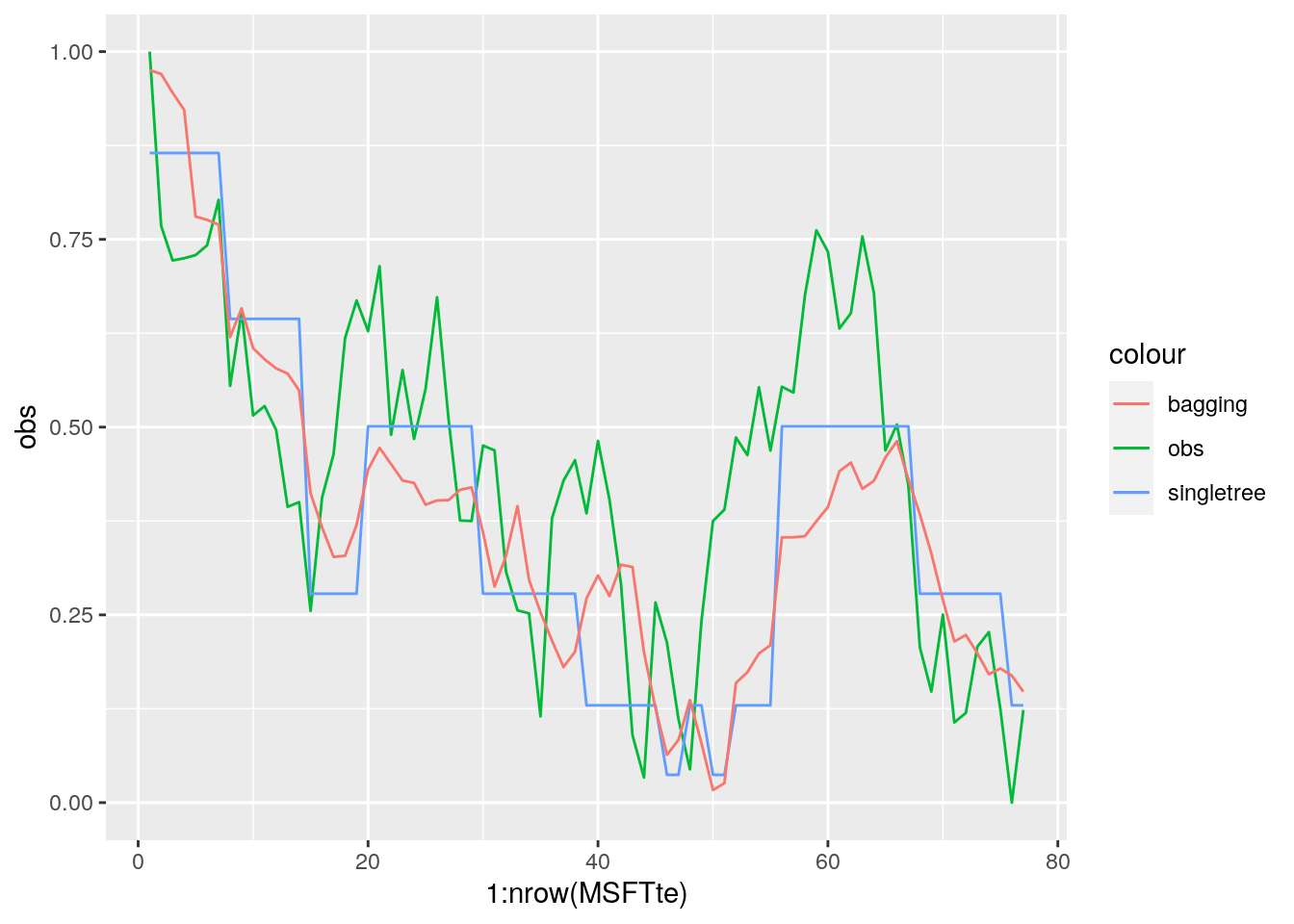
We analyze now graphically the importance of the regressors (this output is obtained by setting importance = T):
varImpPlot(bag)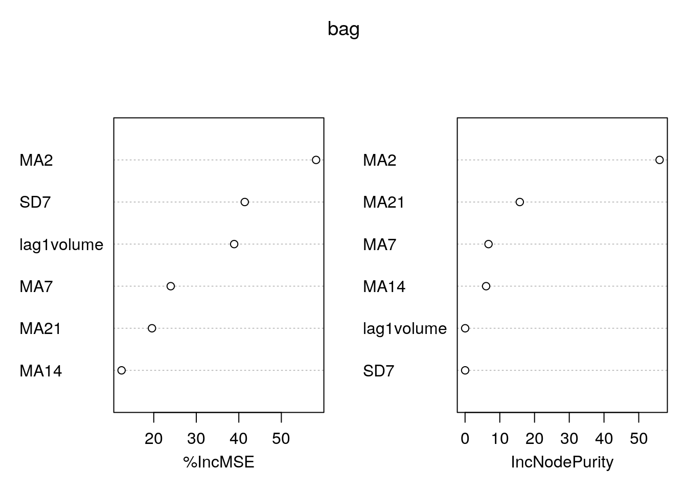
The left plot reports the % increase (averaged across all \(B\) trees) of MSE (computed on the OOB samples) when a given variable is excluded. This measures how much we lose in the predictive capability by excluding each variable. The most important regressor, considering all the \(B\) trees, is MA2.
9.2 Random forest
Random forest is very similar to bagging. The only difference is in the specification
of the mtry argument. For a regression problem we consider a number
of regressors to be selected randomly \(p/3\).
set.seed(15) #procedure is random (bootstrap)
rf = randomForest(target ~ .,
                   data = MSFTtr,
                   mtry = (ncol(MSFTtr)-1) / 3, #p/3
                   ntree = 1000,
                   importance = TRUE)
rf
##
## Call:
## randomForest(formula = target ~ ., data = MSFTtr, mtry = (ncol(MSFTtr) - 1)/3, ntree = 1000, importance = TRUE)
## Type of random forest: regression
## Number of trees: 1000
## No. of variables tried at each split: 2
##
## Mean of squared residuals: 0.0001339149
## % Var explained: 99.82As before we plot the measure for the importance of the regressors:
varImpPlot(rf)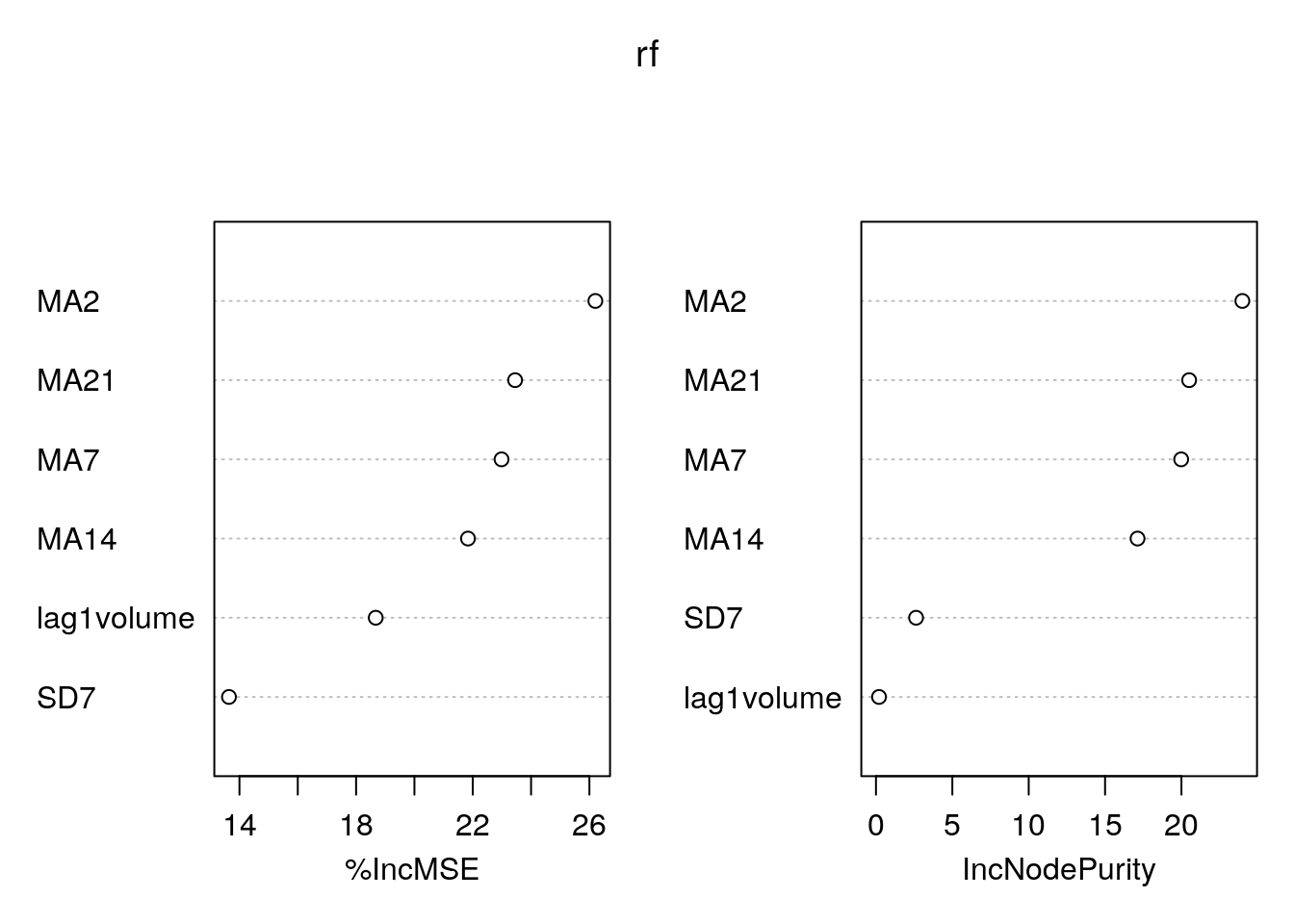 Again
Again MA2 is the most important regressor.
Finally, we compute the predictions and the test MSE by using the random forest model:
pricepred_rf = predict(rf, MSFTte)

MSE_rf = mean((MSFTte$target - pricepred_rf)^2)
MSE_singletree
## [1] 0.03220142MSE_bag## [1] 0.03355776MSE_rf## [1] 0.04388617It results that random forest is performing worse than bagging.
data.frame(obs = MSFTte$target,
           pred_singletree = pricepred,
           pred_bag = pricepred_bag,
           pred_rf = pricepred_rf) %>%
  ggplot() +
  geom_line(aes(1:nrow(MSFTte), obs, col="obs")) +
  geom_line(aes(1:nrow(MSFTte), pred_singletree, col="singletree")) +
  geom_line(aes(1:nrow(MSFTte), pred_bag, col="bagging"))+
  geom_line(aes(1:nrow(MSFTte), pred_rf, col="rf"))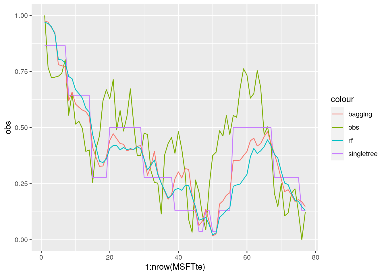
9.3 Gradient boosting
We train a gradient boosting model (gbm) for predicting target by using all the available regressors. Remember that with gbm there are 3 tuning parameters:
- \(B\) the number of trees (i.e. iterations);
- the learning rate or shrinkage parameter \(\lambda\);
- the maximum depth of each tree \(d\) (interaction depth). Note that more than two splitting nodes are required to detect interactions between variables.
We start by setting \(B=5000\) trees (n.trees = 5000), \(\lambda= 0.1\) (shrinkage = 0.1) and \(d=1\) (interaction.depth = 1, i.e. we consider only stumps). In order to study the effect of the tuning parameter \(B\) we will use 5-folds cross-validation. Given that cross-validation is a random procedure we will set the seed before running the function gbm (see also ?gbm). In order to run the gradient boosting method we will have to specify also distribution = "gaussian":
We start setting \(B=1000\), \(d=1\) and \(\lambda=0.1\).
set.seed(15) #cv is random
boost = gbm(target ~ .,
            distribution = "gaussian",
            data = MSFTtr,
            n.trees = 1000, #B
            interaction.depth = 1, #d
            shrinkage = 0.1, #lambda
            cv.folds = 5)
We are now interested in exploring the content of the vector cv.error contained in the output object boost: it contains the values of the CV error (which is an estimate of the test error) for all the values of \(B\) between 1 and 1000. For this reason the length of the vector is equal to \(B\):
length(boost$cv.error)## [1] 1000We want to discover which is the value of \(B\) for which we obtain the lowest value of the CV error:
min(boost$cv.error) #lowest value of the CV error## [1] 0.000205151which.min(boost$cv.error) #corresponding value of B## [1] 952The same output could be obtained by using the gbm.perf function. It returns the value of \(B\) (a value included between 1 and 1000) for which the CV error is lowest. Moreover, it provides a plot with the error as a function of the number of iterations: the black line is the training error while the green line is the CV error, the one we are interested in, the blue line indicates the best value of the number of iterations.
gbm.perf(boost)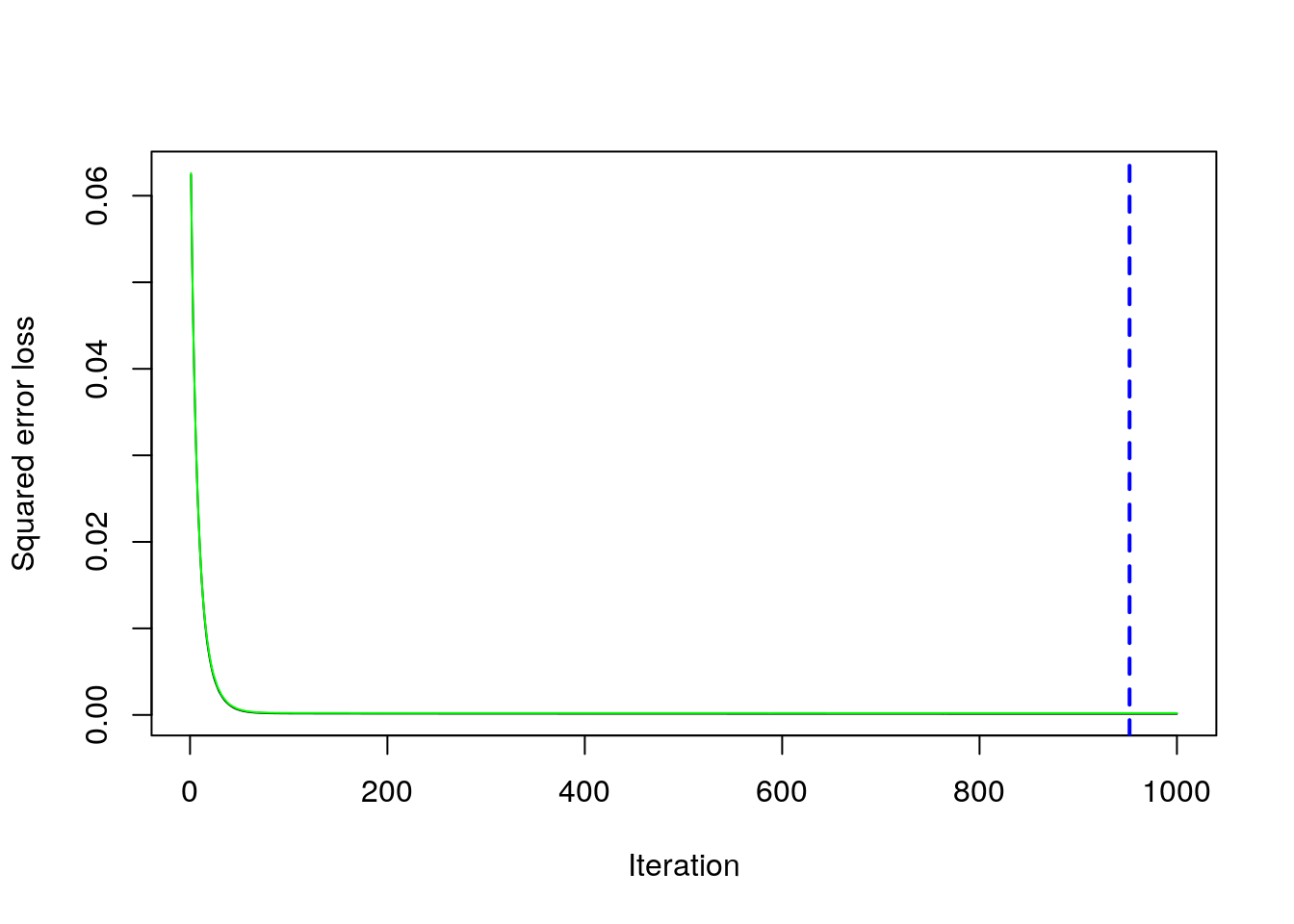
## [1] 9529.3.1 Gradient boosting: parameter tuning
We have found the best value of \(B\) for two fixed values of \(\lambda\) and \(d\). We have to take into account also possible values for them. In particular, we will consider the value c(0.005, .01, .1) for the learning rate \(\lambda\) and c(1, 3, 5) for the tree depth \(d\). We use a for loop to train 9 gradient boosting algorithms according to the 9 combinations of tuning parameters defined by 3 values of \(\lambda\) combined with 3 values of \(d\). As before, we will use the CV error to choose the best combination of \(\lambda\) and \(d\).
We first create a grid of hyperparameters by using the expand_grid function:
grid_par = expand.grid(
  lambda = c(0.005,0.01,0.1),
  d = c(1, 3, 5)
)
grid_par
## lambda d
## 1 0.005 1
## 2 0.010 1
## 3 0.100 1
## 4 0.005 3
## 5 0.010 3
## 6 0.100 3
## 7 0.005 5
## 8 0.010 5
## 9 0.100 5Then we run the for loop with an index i going from 1 to 9 (which is given by nrow(grid_par)). At each iteration of the for loop we use a specific combination of \(\lambda\) and \(d\) taken from hyper_grid. We will finally save the lowest CV error and the corresponding value of \(B\) in new columns of the hyper_grid dataframe:
for(i in 1:nrow(grid_par)){
  set.seed(15) #cv is random
  boost = gbm(target ~ .,
              distribution = "gaussian",
              data = MSFTtr,
              n.trees = 1000, #B
              interaction.depth = grid_par$d[i], #d
              shrinkage = grid_par$lambda[i], #lambda
              cv.folds = 5)

  #the lowest CV error value
  grid_par$CVMSE[i] = min(boost$cv.error)
  # B for which the CV error is lowest
  grid_par$B[i] = which.min(boost$cv.error)
}
We see that now grid_par contains two additional columns (CVMSE and B). It is possible to order the data by using the values contained in the CVMSE column in order to find the best value of \(\lambda\) and \(d\):
grid_par %>%
  arrange(CVMSE)
## lambda d CVMSE B
## 1 0.100 5 0.0001624222 669
## 2 0.100 3 0.0001634308 624
## 3 0.010 5 0.0001634772 1000
## 4 0.010 3 0.0001672920 1000
## 5 0.005 5 0.0001797938 1000
## 6 0.010 1 0.0001869992 1000
## 7 0.005 3 0.0001901395 1000
## 8 0.100 1 0.0002051510 952
## 9 0.005 1 0.0006799117 1000Note that the optimal number of iterations and the learning rate \(\lambda\) depend on each other (the lower the value of \(\lambda\) the higher the number of iterations).
9.3.2 Gradient boosting: final model
Given the best set of hyperparameters, we run the final gbm model (here it would be possible also to choose a higher value of \(B\) to see if we can get any additional improvement in the CV error:
set.seed(15) #cv is random
boost_final = gbm(target ~ .,
            distribution = "gaussian",
            data = MSFTtr,
            n.trees = 1000, #B
            interaction.depth = 5, #d
            shrinkage = 0.1,#lambda
            cv.folds = 5)
boost_best = gbm.perf(boost_final)
We save the best value of \(B\) retrieved by using the gbm.perf function in a new object. This will be needed later for prediction:
boost_best = gbm.perf(boost_final)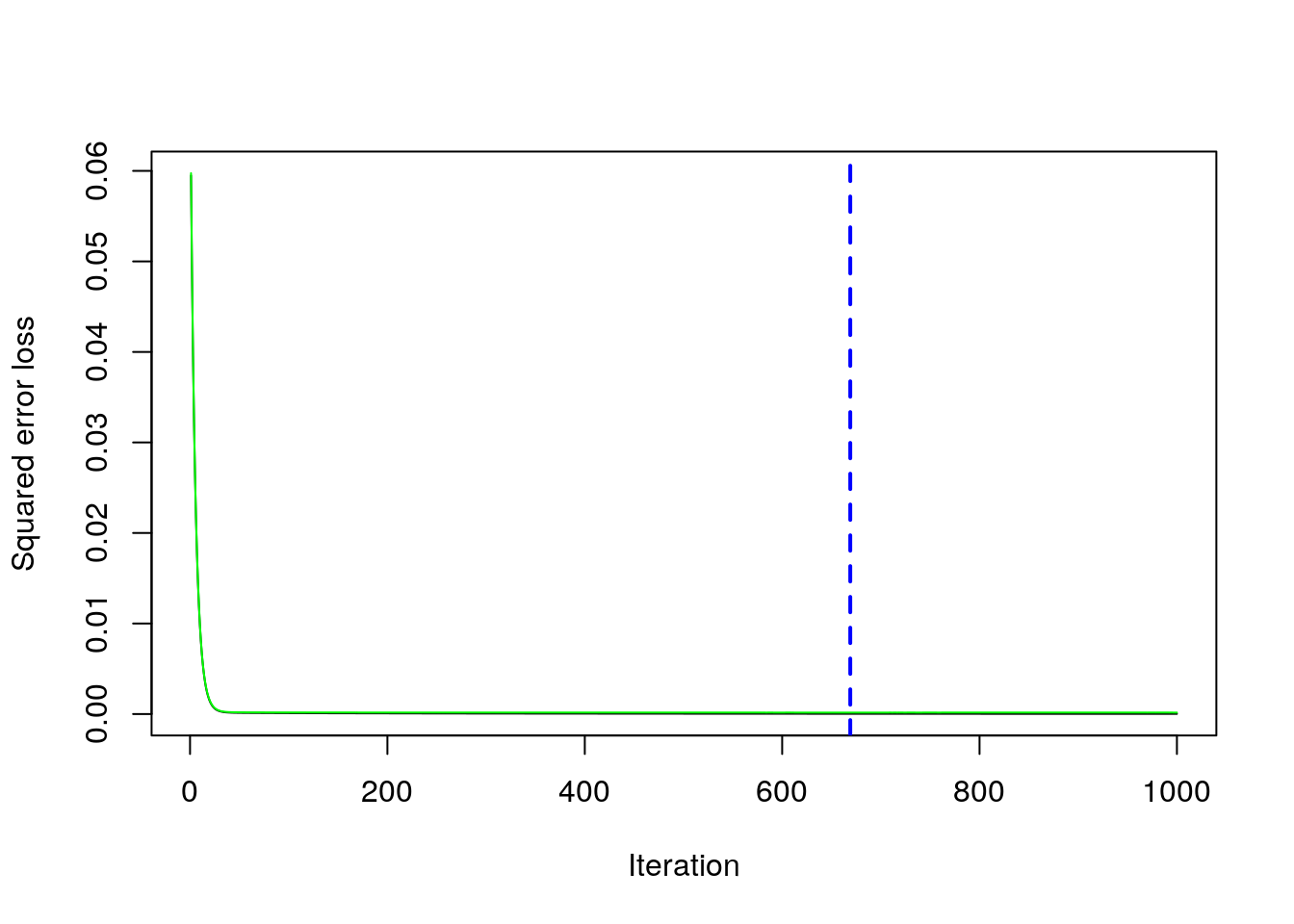
We compute now the prediction for the test data using the standard predict function for which it will be necessary to specify the value of \(B\) that we want to use (boost_best in this case):
pricepred_boost = predict(boost_final,
                          MSFTte,
                          n.trees = boost_best)
It is also possibile to omit n.trees and in this case automatically the value corresponding to the blue line in the gbm.perf plot will be chosen (which is exactly what we are doing, but n.trees can be used more generally for specifying the value of \(B\) that is desired).
Given the prediction we can compute the MSE:
MSE_boosting = mean((MSFTte$target - pricepred_boost)^2)
MSE_boosting
## [1] 0.03114458MSE_singletree## [1] 0.03220142MSE_bag## [1] 0.03355776MSE_rf## [1] 0.04388617We see that boosting performs better than the other methods (it has the lowest test MSE). Still it is not able to completely catch the values of the observed time series (though it can predict the trend).
We finally compare all the predicted time series:
# plot the observed and the predicted values
data.frame(obs = MSFTte$target,
           pred_singletree = pricepred,
           pred_bag = pricepred_bag,
           pred_rf = pricepred_rf,
           pred_boost = pricepred_boost) %>%
  ggplot() +
  geom_line(aes(1:nrow(MSFTte), obs, col="obs")) +
  geom_line(aes(1:nrow(MSFTte), pred_singletree, col="singletree")) +
  geom_line(aes(1:nrow(MSFTte), pred_bag, col="bagging"))+
  geom_line(aes(1:nrow(MSFTte), pred_rf, col="rf"))+
  geom_line(aes(1:nrow(MSFTte), pred_boost, col="boosting"))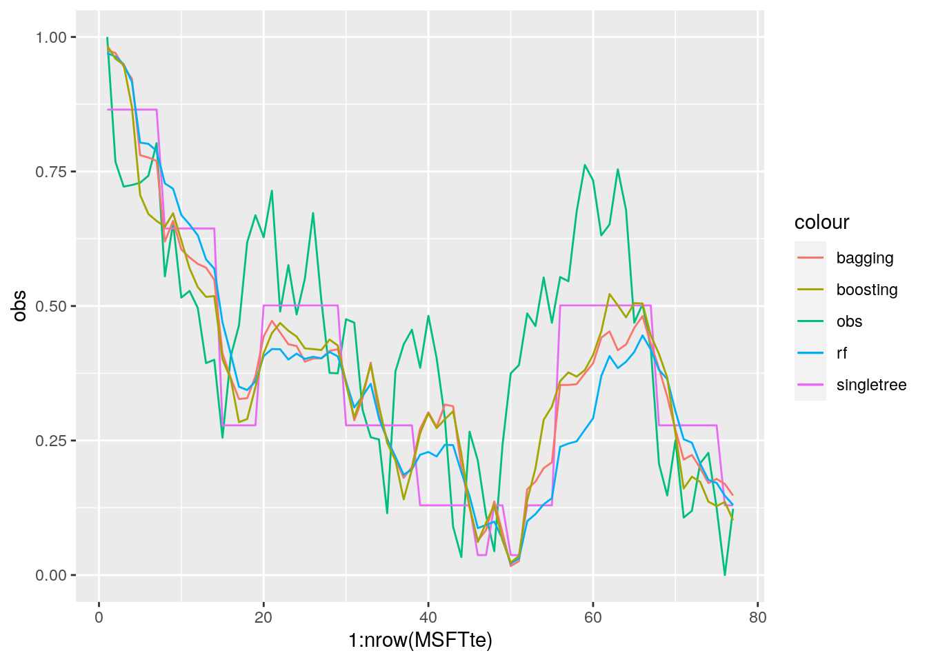
Given that boosting is the best model, we compute also the correlation between the observed time series values and the boosting predictions:
cor(pricepred_boost, MSFTte$target)## [1] 0.70819469.4 Exercises Lab 7
9.4.1 Exercise 1
Consider the bike sharing data used for Lab. 4 (the file is called bikesharing.csv and it’s available in the e-learning). Explore the dataset. The response variable is cnt (count of total rental bikes including both casual and registered users). All the other variables but registered will be used as regressors.
Remove
registeredandcasualfrom the dataframe (ascnt=casual+registered). Remove alsodtedaywhich is a character variable with the date strings.Split the original data set into a training (70%) and test set. Use 44 as seed. Moreove, compute the average number of rental bikes for the two datasets.
Implement bagging to predict
cnt(use 44 as seed and 1000 trees). Compute also the test MSE for bagging.Implement random forest (use 44 as seed) for the same set of data and compare its performance (in terms of MSE) with the method implemented before.
Implement gradient boosting for the same set of data by using \(B=5000\), \(d=1\) and \(\lambda=0.1\) and 5-folds cross-validation. Use 44 as seed. Which is the best value of \(B\) for this specific parameter setting?
In order to tune the value of the hyperparameter consider the values
c(0.005, .01, .1, 0.2)for the learning rate \(\lambda\) andc(1, 3, 5, 7)for the tree depth (use \(B=5000\)). Implement a for loop to iterate across the 16 parameters’ combinations. Which is the best setting for \(\lambda\) and \(d\)?Given the parameter values chosen at the previous point, rerun gbm by using \(B=7000\). Then detect the best value of \(B\) and compute the final predictions for the test set and the corresponding MSE.
Compare bagging, random forest and gb in terms of MSE? Which method does perform better? Study the importance of the variable for the best model.
Given the best method, plot predicted and observed values for
cnt. For setting the color of the points use theseasonvariable.
9.4.2 Exercise 2
Consider Exercise 1 of Lab 6, referring to file Adjcloseprices.csv: it contains the adjusted close prices for Apple (AAPL) and the values of the NASDAQ index (IXIC). There is also a column containing dates). Rerun all the data transformation implemented for Lab 6, and then compare the single tree model with bagging, random forest and boosting. Which is the best method for predicting the future values of the APPLE prices time series?