Chapter 7 R Lab 5 - 13/04/2022
In this lecture we will learn how to implement the linear and the quadratic discriminant analysis (LDA and QDA) and the Naive Bayes method. Moreover, the methods will be compared by using performance indexes and the ROC curve.
The following packages are required: MASS, naivebayes, pROC and tidyverse.
library(MASS) #for LDA and QDA##
## Attaching package: 'MASS'## The following object is masked from 'package:dplyr':
##
## selectlibrary(naivebayes) #for naive Bayes classifier## naivebayes 0.9.7 loadedlibrary(pROC) #for ROC curve## Type 'citation("pROC")' for a citation.##
## Attaching package: 'pROC'## The following objects are masked from 'package:stats':
##
## cov, smooth, varlibrary(tidyverse)7.1 Loan default data
The data we use for this lab are taken from the book titled “Machine Learning & Data Science Blueprints for Finance” (suggested for the AIMLFF course). See in particular the Case Study 2: loan default probability in Chapter 6. The goal is to build machine learning models to predict the probability that a loan will default and won’t be repaid by the borrower.
The response variable is named charged_off and is a binary variable: 0 means that the borrower was able to fully pay the loan, while 1 means that the loan was charged off (default). In this case study there are several regressors, both quantitative and qualitative.
We import the data as usual
data <- read.csv("./files/loandefault.csv")
glimpse(data)
## Rows: 86,138
## Columns: 34
## $ loan_amnt <dbl> 15000, 10400, 21425, 7650, 9600, 2500, 16000, 23…
## $ funded_amnt <dbl> 15000, 10400, 21425, 7650, 9600, 2500, 16000, 23…
## $ term <fct> 60 months, 36 months, 60 months, 36 months, …
## $ int_rate <dbl> 12.39, 6.99, 15.59, 13.66, 13.66, 11.99, 11.44, …
## $ installment <dbl> 336.64, 321.08, 516.36, 260.20, 326.53, 83.03, 3…
## $ grade <fct> C, A, D, C, C, B, B, C, B, B, D, C, B, C, B, D, …
## $ sub_grade <fct> C1, A3, D1, C3, C3, B5, B4, C4, B4, B5, D5, C3, …
## $ emp_title <fct> "MANAGEMENT", "Truck Driver Delivery Personel", …
## $ emp_length <fct> 10+ years, 8 years, 6 years, < 1 year, 10+ years…
## $ home_ownership <fct> RENT, MORTGAGE, RENT, RENT, RENT, MORTGAGE, OWN,…
## $ annual_inc <dbl> 78000, 58000, 63800, 50000, 69000, 89000, 109777…
## $ verification_status <fct> Source Verified, Not Verified, Source Verified, …
## $ purpose <fct> debt_consolidation, credit_card, credit_card, de…
## $ title <fct> Debt consolidation, Credit card refinancing, Cre…
## $ zip_code <fct> 235xx, 937xx, 658xx, 850xx, 077xx, 554xx, 201xx,…
## $ addr_state <fct> VA, CA, MO, AZ, NJ, MN, VA, WA, MD, MI, FL, NY, …
## $ dti <dbl> 12.03, 14.92, 18.49, 34.81, 25.81, 13.77, 11.63,…
## $ earliest_cr_line <fct> Aug-1994, Sep-1989, Aug-2003, Aug-2002, Nov-1992…
## $ fico_range_low <dbl> 750, 710, 685, 685, 680, 685, 700, 665, 745, 675…
## $ fico_range_high <dbl> 754, 714, 689, 689, 684, 689, 704, 669, 749, 679…
## $ open_acc <dbl> 6, 17, 10, 11, 12, 9, 7, 14, 8, 5, 11, 7, 11, 10…
## $ revol_util <dbl> 29.0, 31.6, 76.2, 91.9, 59.4, 94.3, 60.4, 82.2, …
## $ initial_list_status <fct> w, w, w, f, f, f, w, f, f, f, f, f, f, f, f, f, …
## $ last_pymnt_amnt <dbl> 12017.81, 321.08, 17813.19, 17.70, 9338.58, 2294…
## $ application_type <fct> Individual, Individual, Individual, Individual, …
## $ acc_open_past_24mths <dbl> 5, 7, 4, 6, 8, 6, 3, 6, 4, 0, 7, 2, 5, 6, 2, 6, …
## $ avg_cur_bal <dbl> 29828, 9536, 4232, 5857, 3214, 44136, 53392, 393…
## $ bc_open_to_buy <dbl> 9525, 7599, 324, 332, 6494, 1333, 2559, 3977, 12…
## $ bc_util <dbl> 4.7, 41.5, 97.8, 93.2, 69.2, 86.4, 72.2, 89.0, 2…
## $ mo_sin_old_rev_tl_op <dbl> 244, 290, 136, 148, 265, 148, 133, 194, 67, 124,…
## $ mo_sin_rcnt_rev_tl_op <dbl> 1, 1, 7, 8, 23, 24, 17, 15, 12, 40, 2, 21, 15, 8…
## $ mort_acc <dbl> 0, 1, 0, 0, 0, 5, 2, 6, 0, 0, 0, 2, 5, 0, 0, 0, …
## $ num_actv_rev_tl <dbl> 4, 9, 4, 4, 7, 4, 3, 5, 2, 5, 8, 3, 8, 6, 3, 2, …
## $ charged_off <int> 0, 1, 0, 1, 0, 0, 0, 1, 0, 1, 1, 0, 0, 0, 0, 0, …7.2 Data preparation
The following steps follows the approach used in the book. As we will implement LDA and QDA, we need to have only quantitative regressors. They can be jointly selected by using the function select_if (we create a new dataframe called data2):
data2 = data %>% select_if(is.numeric)
glimpse(data2)
## Rows: 86,138
## Columns: 20
## $ loan_amnt <dbl> 15000, 10400, 21425, 7650, 9600, 2500, 16000, 23…
## $ funded_amnt <dbl> 15000, 10400, 21425, 7650, 9600, 2500, 16000, 23…
## $ int_rate <dbl> 12.39, 6.99, 15.59, 13.66, 13.66, 11.99, 11.44, …
## $ installment <dbl> 336.64, 321.08, 516.36, 260.20, 326.53, 83.03, 3…
## $ annual_inc <dbl> 78000, 58000, 63800, 50000, 69000, 89000, 109777…
## $ dti <dbl> 12.03, 14.92, 18.49, 34.81, 25.81, 13.77, 11.63,…
## $ fico_range_low <dbl> 750, 710, 685, 685, 680, 685, 700, 665, 745, 675…
## $ fico_range_high <dbl> 754, 714, 689, 689, 684, 689, 704, 669, 749, 679…
## $ open_acc <dbl> 6, 17, 10, 11, 12, 9, 7, 14, 8, 5, 11, 7, 11, 10…
## $ revol_util <dbl> 29.0, 31.6, 76.2, 91.9, 59.4, 94.3, 60.4, 82.2, …
## $ last_pymnt_amnt <dbl> 12017.81, 321.08, 17813.19, 17.70, 9338.58, 2294…
## $ acc_open_past_24mths <dbl> 5, 7, 4, 6, 8, 6, 3, 6, 4, 0, 7, 2, 5, 6, 2, 6, …
## $ avg_cur_bal <dbl> 29828, 9536, 4232, 5857, 3214, 44136, 53392, 393…
## $ bc_open_to_buy <dbl> 9525, 7599, 324, 332, 6494, 1333, 2559, 3977, 12…
## $ bc_util <dbl> 4.7, 41.5, 97.8, 93.2, 69.2, 86.4, 72.2, 89.0, 2…
## $ mo_sin_old_rev_tl_op <dbl> 244, 290, 136, 148, 265, 148, 133, 194, 67, 124,…
## $ mo_sin_rcnt_rev_tl_op <dbl> 1, 1, 7, 8, 23, 24, 17, 15, 12, 40, 2, 21, 15, 8…
## $ mort_acc <dbl> 0, 1, 0, 0, 0, 5, 2, 6, 0, 0, 0, 2, 5, 0, 0, 0, …
## $ num_actv_rev_tl <dbl> 4, 9, 4, 4, 7, 4, 3, 5, 2, 5, 8, 3, 8, 6, 3, 2, …
## $ charged_off <int> 0, 1, 0, 1, 0, 0, 0, 1, 0, 1, 1, 0, 0, 0, 0, 0, …The next step is to transform the response variable (now coded as 0/1 integer variable) into a factor with categories 0_Fully Paid and 1_Charged Off. Note that we check the frequency distribution of the variable charged_off before and after the transformation to be sure that everything works fine:
table(data2$charged_off)##
## 0 1
## 69982 16156# from integer to factor
data2$charged_off = factor(data2$charged_off,
levels = c(0,1),
labels = c("0_Fully Paid", "1_Charged Off"))
table(data2$charged_off)##
## 0_Fully Paid 1_Charged Off
## 69982 16156If we run the summary function we realize that some of the variables have missing values (e.g. bc_open_to_buy):
summary(data2)## loan_amnt funded_amnt int_rate installment
## Min. : 1000 Min. : 1000 Min. : 6.00 Min. : 30.42
## 1st Qu.: 7800 1st Qu.: 7800 1st Qu.: 9.49 1st Qu.: 248.48
## Median :12000 Median :12000 Median :12.99 Median : 370.48
## Mean :14107 Mean :14107 Mean :13.00 Mean : 430.74
## 3rd Qu.:20000 3rd Qu.:20000 3rd Qu.:15.61 3rd Qu.: 568.00
## Max. :35000 Max. :35000 Max. :26.06 Max. :1408.13
##
## annual_inc dti fico_range_low fico_range_high
## Min. : 4000 Min. : 0.00 Min. :660.0 Min. :664.0
## 1st Qu.: 45000 1st Qu.:12.07 1st Qu.:670.0 1st Qu.:674.0
## Median : 62474 Median :17.95 Median :685.0 Median :689.0
## Mean : 73843 Mean :18.53 Mean :692.5 Mean :696.5
## 3rd Qu.: 90000 3rd Qu.:24.50 3rd Qu.:705.0 3rd Qu.:709.0
## Max. :7500000 Max. :39.99 Max. :845.0 Max. :850.0
##
## open_acc revol_util last_pymnt_amnt acc_open_past_24mths
## Min. : 1.00 Min. : 0.00 Min. : 0.0 Min. : 0.000
## 1st Qu.: 8.00 1st Qu.: 37.20 1st Qu.: 358.5 1st Qu.: 2.000
## Median :11.00 Median : 54.90 Median : 1241.2 Median : 4.000
## Mean :11.75 Mean : 54.58 Mean : 4757.4 Mean : 4.595
## 3rd Qu.:14.00 3rd Qu.: 72.50 3rd Qu.: 7303.2 3rd Qu.: 6.000
## Max. :84.00 Max. :180.30 Max. :36234.4 Max. :53.000
## NA's :44
## avg_cur_bal bc_open_to_buy bc_util mo_sin_old_rev_tl_op
## Min. : 0 Min. : 0 Min. : 0.00 Min. : 3.0
## 1st Qu.: 3010 1st Qu.: 1087 1st Qu.: 44.10 1st Qu.:118.0
## Median : 6994 Median : 3823 Median : 67.70 Median :167.0
## Mean : 13067 Mean : 8943 Mean : 63.81 Mean :183.5
## 3rd Qu.: 17905 3rd Qu.: 10588 3rd Qu.: 87.50 3rd Qu.:232.0
## Max. :447433 Max. :249625 Max. :255.20 Max. :718.0
## NA's :996 NA's :1049
## mo_sin_rcnt_rev_tl_op mort_acc num_actv_rev_tl charged_off
## Min. : 0.0 Min. : 0.000 Min. : 0.000 0_Fully Paid :69982
## 1st Qu.: 3.0 1st Qu.: 0.000 1st Qu.: 3.000 1_Charged Off:16156
## Median : 8.0 Median : 1.000 Median : 5.000
## Mean : 12.8 Mean : 1.749 Mean : 5.762
## 3rd Qu.: 15.0 3rd Qu.: 3.000 3rd Qu.: 7.000
## Max. :372.0 Max. :34.000 Max. :38.000
## One possibility is to do data imputation for the missing values. Here instead we will remove the observations with one or more than one missing values by using na.omit:
data3 = na.omit(data2)Note the reduction in the number of observation for data3 when removing the missing values from data2.
From the preview of the data and the summary statistics we realize that loan_amnt and funded_amnt have the same values. To be sure that these two variables take exactly the same values we compute the differences and then summarize them by using the sum:
sum(data3$loan_amnt - data3$funded_amnt)## [1] 0As the sum is exactly equal to zero it means that the two columns are exactly the same. Thus, we need to remove one of the two for avoiding problems with the models’ estimation:
# Remove funded_amnt
data3 = data3 %>% dplyr::select(-funded_amnt)
We then plot the distribution of annual_inc conditionally on charged_off by using boxplots:
data3 %>%
  ggplot()+
  geom_boxplot(aes(charged_off,
                   annual_inc))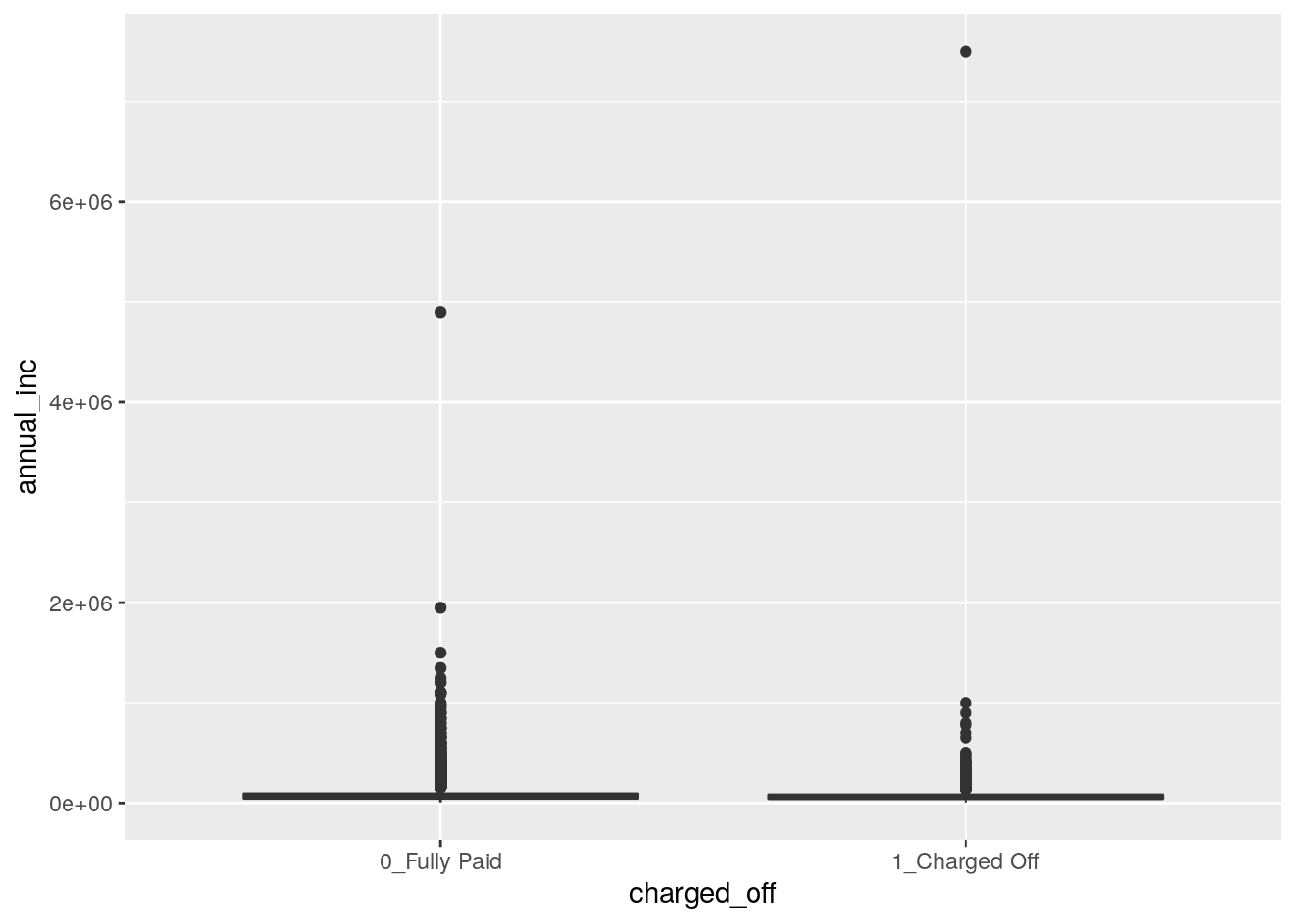
We see that, due to the extreme values in the annual_inc the boxes are completely hidden and the distribution of the variable is not clearly shown. We try to apply the log transformation to the quantitative variable:
data3 %>%
  ggplot()+
  geom_boxplot(aes(charged_off,
                   log(annual_inc)))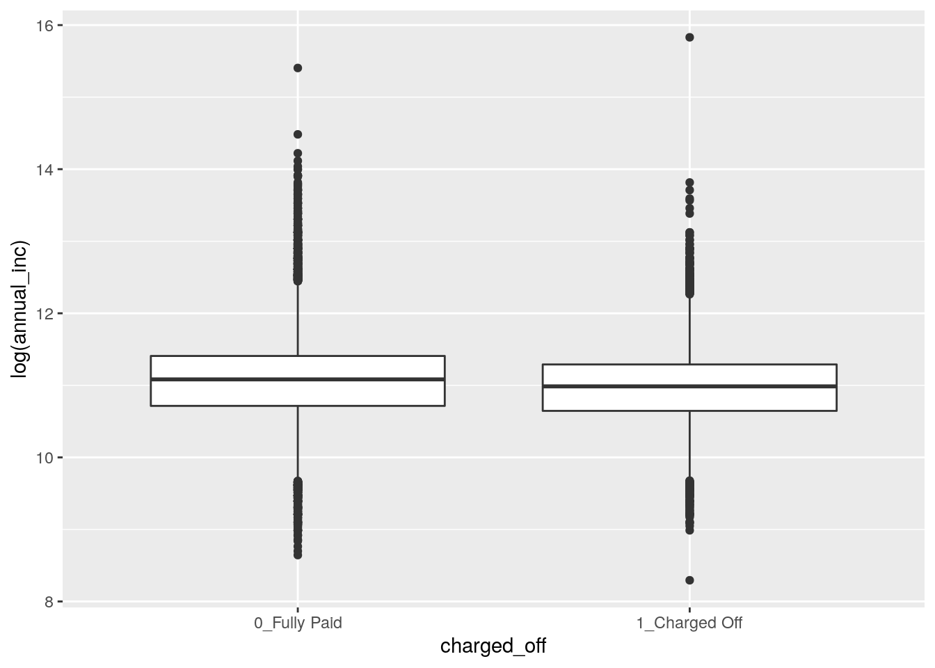
Now, the distribuion appears more reasonable for both the categories (the median annual_inc is very similar in the two groups). We thus decise to apply this transformation permanently in the dataframe by substitution:
data3 = data3 %>%
  mutate(annual_inc = log(annual_inc))
We check now the correlation between the fico_range_high and fico_range_low, where the FICO score is designed to rank-order consumers by their sensitivity to a future economic downturn.
cor(data3$fico_range_high,
    data3$fico_range_low)
## [1] 1The correlation is exactly equal to one meaning that the two variables are perfectly linearly associated, see also the following plot:
data3 %>%
  ggplot()+
  geom_point(aes(fico_range_high,
                  fico_range_low))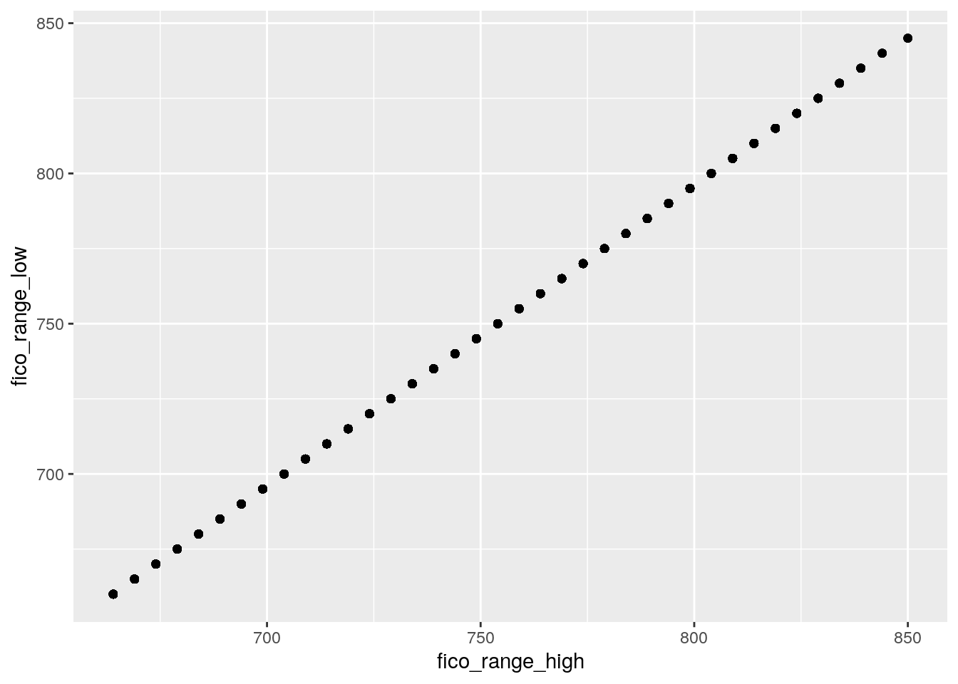
This means that it doesn’t make sense to have both the variables for the modeling because they provide the same information. We thus create a new variable which is the average of the two (remember to remove the original variables after the creation of fico_new):
data3 = data3 %>%
  mutate(fico_new = (fico_range_high+fico_range_low)/2) %>%
  dplyr::select(-fico_range_high, -fico_range_low)
7.3 A new method for creating the training and testing set
To create the training (80%) and test (20%) dataset we use a new approach different from the one introduced in Section 6.1.1.
We first create a vector with the indexes we will use for the training dataset. In this case we must set replace to false, since each index will indicate an observation belonging just to the training or test set. Recall also to set a seed, in order to be able to replicate your results:
set.seed(56)
train_indexes = sample(1:nrow(data3),
                       0.8*nrow(data3),
                       replace = FALSE)
head(train_indexes) #positions
## [1] 47264 47907 72102 10502 33471 30038We are now ready to sample from the data3 dataset 80% of the observations (rows) by using the train_index vector, and leave the non-sampled indexes for test. Just use a minus (-) before the row selection to exclude them:
# recall: dataset [ row , columns ]
training = data3[train_indexes,]
test = data3[-train_indexes,]
Note that this procedure could be the easiest choice when we don’t have a third dataset (validation).
We are now ready to train our models.
7.4 Definition of a function for computing performance indexes
For assessing the performance of a classifier we compare predicted categories with observed categories. This can be done by using the confusion matrix which is a 2x2 matrix reporting the joint distribution (with absolute frequencies) of predicted (by row) and observed (by column) categories.
| No (obs.) | Yes (obs.) | |||
|---|---|---|---|---|
| No (pred.) | TN | FN | ||
| Yes (pred.) | FP | TP | ||
| Total | N | P |
We consider in particular the following performance indexes:
- sensitivity (true positive rate): TP/P
- specificity (true negative rate): TN/N
- accuracy (rate of correctly classified observations): (TN+TP)/(N+P)
We define a function named perf_indexes which computes the above defined indexes. The function has only one argument which is a confusion 2x2 matrix named cm. It returns a vector with the 3 indexes.
perf_indexes = function(cm){
  sensitivity = cm[2,2] / (cm[1,2] + cm[2,2])
  specificity = cm[1,1] / (cm[1,1] + cm[2,1])
  accuracy = sum(diag(cm)) / sum(cm)
  return(c(sens=sensitivity,spec=specificity,acc=accuracy))
}
7.5 Linear discriminant analysis (LDA)
To run LDA we use the lda function of the MASS package. We have to specify the formula and the data:
ldamod = lda(charged_off ~ ., data = training)
ldamod
## Call:
## lda(charged_off ~ ., data = training)
##
## Prior probabilities of groups:
## 0_Fully Paid 1_Charged Off
## 0.8139149 0.1860851
##
## Group means:
## loan_amnt int_rate installment annual_inc dti open_acc
## 0_Fully Paid 13904.86 12.38479 428.0233 11.07335 18.03627 11.68787
## 1_Charged Off 15189.28 15.57432 448.6859 10.97801 20.71857 12.22697
## revol_util last_pymnt_amnt acc_open_past_24mths avg_cur_bal
## 0_Fully Paid 53.79476 5767.4285 4.448506 13497.27
## 1_Charged Off 57.80569 462.1843 5.296045 10528.62
## bc_open_to_buy bc_util mo_sin_old_rev_tl_op
## 0_Fully Paid 9495.520 62.77151 185.9586
## 1_Charged Off 6585.875 68.24895 173.7827
## mo_sin_rcnt_rev_tl_op mort_acc num_actv_rev_tl fico_new
## 0_Fully Paid 13.04113 1.799780 5.685113 696.3214
## 1_Charged Off 10.93337 1.484724 6.281677 686.9207
##
## Coefficients of linear discriminants:
## LD1
## loan_amnt 2.650323e-04
## int_rate 1.372393e-01
## installment -6.348282e-03
## annual_inc -5.780011e-02
## dti 6.631218e-03
## open_acc -5.827416e-03
## revol_util -8.716455e-05
## last_pymnt_amnt -1.807028e-04
## acc_open_past_24mths 5.176170e-02
## avg_cur_bal -1.304181e-06
## bc_open_to_buy -7.834754e-08
## bc_util -3.082502e-04
## mo_sin_old_rev_tl_op -3.882009e-04
## mo_sin_rcnt_rev_tl_op 1.679736e-04
## mort_acc -1.528716e-02
## num_actv_rev_tl -1.716518e-03
## fico_new -1.226463e-03The output reports the prior probabilities (\(\hat \pi_k\)) for the two categories and the conditional means of all the covariates (\(\hat \mu_k\)). Recall that the prior probability is the probability that a randomly chosen observation comes from the \(k\)-th class.
We go straight to the calculation of the predictions:
ldamodpred = predict(ldamod, newdata = test)
names(ldamodpred)
## [1] "class" "posterior" "x"Note that the object ldamodpred is a list containing 3 objects including the vector of posterior probabilities (posterior) and the vector of predicted categories (`class):
head(ldamodpred$posterior)## 0_Fully Paid 1_Charged Off
## 5 0.9838726 0.01612736
## 10 0.9159457 0.08405434
## 13 0.9571846 0.04281537
## 16 0.8780302 0.12196976
## 17 0.8980612 0.10193884
## 22 0.9316872 0.06831281head(ldamodpred$class)## [1] 0_Fully Paid 0_Fully Paid 0_Fully Paid 0_Fully Paid 0_Fully Paid
## [6] 0_Fully Paid
## Levels: 0_Fully Paid 1_Charged OffNote that the predictions contained in ldamodpred$class are computed using as threshold for the posterior probabilities the value 0.5 (standard choice).
To compute the confusion matrix we will use the vector ldamodpred$class:
table(ldamodpred$class, test$charged_off)##
## 0_Fully Paid 1_Charged Off
## 0_Fully Paid 13444 1869
## 1_Charged Off 312 1393perf_indexes(table(ldamodpred$class, test$charged_off))## sens spec acc
## 0.4270386 0.9773190 0.8718416Note that the value of the sensitivity (true positive rate) is quite low, while specificity and accuracy are quite high. It seems that LDA is not able to correctly identify the actual defaulters.
We could choose a different threshold for our decision. In this case, the used functions do not allow to change directly the threshold. Recall that LDA assign the the observation to the majority class (= class with highest posterior probability). So, there is an implicit probability threshold with two classes (\(0.5\)). Check it by yourself here below:
ldapred_myclass = ifelse(ldamodpred$posterior[,"1_Charged Off"] > 0.5,
                         "1_Charged Off",
                         "0_Fully Paid")
# same results than in the previous LDA
table(ldapred_myclass, test$charged_off)
##
## ldapred_myclass 0_Fully Paid 1_Charged Off
## 0_Fully Paid 13444 1869
## 1_Charged Off 312 1393# same results than in the previous LDA
perf_indexes(table(ldapred_myclass, test$charged_off))## sens spec acc
## 0.4270386 0.9773190 0.8718416We can now set an higher probability threshold, with the aim of being able to better select the “real” default customers. Let’s consider for example a value of the probability threshold equal to \(0.2\) :
lda_pred_myclass2 = ifelse(ldamodpred$posterior[,"1_Charged Off"] > 0.2,
                           "1_Charged",
                           "0_Fully Paid")

table(lda_pred_myclass2, test$charged_off)
##
## lda_pred_myclass2 0_Fully Paid 1_Charged Off
## 0_Fully Paid 11778 966
## 1_Charged 1978 2296perf_indexes(table(lda_pred_myclass2, test$charged_off)) ## sens spec acc
## 0.7038627 0.8562082 0.8270067We are now able to correctly detect more real charged off customers (from \(838\) to \(2296\)), increasing the sensitivity of our algorithm. Specificity and accuracy are slightly reduced.
7.6 Quadratic discriminant analysis (QDA)
QDA works very similar to LDA. We first estimate the model, then get the predictions and finally compute the performance indexes.
qdamod = qda(charged_off ~ .,
             data = training)

# prediction
qdamodpred = predict(qdamod,
                     newdata = test)

# check the performance
# confusion matrix
table(pred = qdamodpred$class, obs = test$charged_off)
## obs
## pred 0_Fully Paid 1_Charged Off
## 0_Fully Paid 9951 238
## 1_Charged Off 3805 3024perf_indexes(table(pred = qdamodpred$class,
obs = test$charged_off))## sens spec acc
## 0.9270386 0.7233934 0.7624280We see that, by using the 0.5 probability threshold, QDA outperforms LDA in terms of sensitivity, while specificity and accuracy are lower.
7.7 Naive Bayes
The function naive_bayes from the naivebayes package is used to compute the posterior probabilities for the two classes and the final most likely class.
nbmod = naive_bayes(formula=charged_off~.,
                     data=training,
                     usekernel = TRUE)
Note that the option usekernel = TRUE is used in order to estimate the density \(\hat f_{jk}\) by using the kernel density estimate (smoothed version of the histogram).
We move on by computing predictions, as done with LDA and QDA:
nbmodpred = predict(nbmod, newdata=test)## Warning: predict.naive_bayes(): more features in the newdata are provided as
## there are probability tables in the object. Calculation is performed based on
## features to be found in the tables.head(nbmodpred)## [1] 0_Fully Paid 0_Fully Paid 0_Fully Paid 0_Fully Paid 0_Fully Paid
## [6] 0_Fully Paid
## Levels: 0_Fully Paid 1_Charged OffThe warning message that we get is not important (it is just saying that in the test dataset there are additional variables that weren’t used as regressors in the training, in this case it is reffering to charged_off which is actually our response variable). Note that in this case nbmodpred is not a list (as with LDA and QDA) but a vector of the predicted categories. If you are interested in the posterior probabilities run the following code:
nbmodpred_prob <- predict(nbmod,
                   newdata=test,
                   type = "prob")
## Warning: predict.naive_bayes(): more features in the newdata are provided as
## there are probability tables in the object. Calculation is performed based on
## features to be found in the tables.head(nbmodpred_prob)## 0_Fully Paid 1_Charged Off
## [1,] 0.9979356 0.002064418
## [2,] 0.5063463 0.493653683
## [3,] 0.8805417 0.119458301
## [4,] 0.9198832 0.080116830
## [5,] 0.6414885 0.358511539
## [6,] 0.9951038 0.004896215We are now ready to evaluate the performance of Naive Bayes:
table(nbmodpred, test$charged_off)##
## nbmodpred 0_Fully Paid 1_Charged Off
## 0_Fully Paid 11523 1224
## 1_Charged Off 2233 2038perf_indexes(table(nbmodpred, test$charged_off))## sens spec acc
## 0.6247701 0.8376708 0.7968621Sensitivity is higher than LDA but lower than QDA. Specificity is lower than LDA but higher than QDA. The accuracy is quite similar to QDA.
7.8 Construction and plotting of the ROC curve
To obtain the ROC curve we use the function roc contained in the pROC package. It is necessary to specify as arguments the vector of the observed categories (response) and the vector of the posterior probabilities for the Yes/positive/1_Charged Off category (predictor).
roc_lda = roc(response = test$charged_off,
              predictor = ldamodpred$posterior[,2])
## Setting levels: control = 0_Fully Paid, case = 1_Charged Off## Setting direction: controls < casesroc_qda = roc(response = test$charged_off,
predictor = qdamodpred$posterior[,2])## Setting levels: control = 0_Fully Paid, case = 1_Charged Off
## Setting direction: controls < casesroc_nb = roc(response = test$charged_off,
predictor = nbmodpred_prob[,2])## Setting levels: control = 0_Fully Paid, case = 1_Charged Off
## Setting direction: controls < casesGiven the ROC curve it is possible to plot it and to compute the area under the curve (auc):
auc(roc_lda)## Area under the curve: 0.8807auc(roc_qda)## Area under the curve: 0.9176auc(roc_nb)## Area under the curve: 0.8451The best method, according to AUC, is QDA as it has the highest AUC value.
ggroc(list(lda = roc_lda,
           qda = roc_qda,
           nb = roc_nb))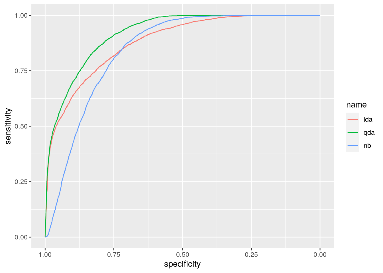
This result is confirmed by the ROC curves, where we observe that the green curve (QDA) dominates the others (and it is located closer to the ideal classifier, in the top left corner).
Note that the plot uses specificity on the x-axis (which goes from 1 on the left to zero on the right) and sensitivity on the y-axis.
7.9 Exercises Lab 5
7.9.1 Exercise 1
The data contained in the files titanic_tr.csv (for training) and titanic_te.csv (and testing) are about the Titanic disaster (the files are available in the e-learning). In particular the following variables are available:
pclass: ticket class (1 = 1st, 2 = 2nd, 3 = 3rd)survived: survival (0 = No, 1 = Yes)nameof the passengersexagein years
sibsp: number of siblings / spouses aboard the Titanic
parchnumber of parents / children aboard the Titanic
ticket: ticket number
fare: passenger fare
cabin: cabin number
embarked: port of Embarkation (C = Cherbourg, Q = Queenstown, S = Southampton)
Import the data in R and explore them. Note that the response variable is survived which is classified as a int 0/1 variable in the dataframe. Transform it in a factor type object using the factor function with categories “No” and “Yes”.
Convert
pclass(ticket class) to factor (1 = “1st”, 2 = “2nd”, 3 = “3rd”) for both the training and test data set. Plotsurvivedas a function ofpclass. In which class do you observe the highest proportion of survivors?Check how many missing values we have in the variables
ageandfareseparately for training and test data.
- Separately for the training and test data, substitute the missing values with the average of
ageandfare. Note that for computing the mean when you have missing values you have to runmean(...,na.rm=T). After this, check that you don’t have any other missing values.
Consider the training data and
survivedas response variable. Compute the percentage of survived people. Moreover, represent graphically the relationship betweenageandsurvived. Comment the plot.Consider the training data set, estimate LDA for
survivedconsideringage,fareandpclassas predictors. Compute the total test classification error.Consider the training data set, estimate QDA for
survivedconsideringage,fareandpclassas predictors. Compute the total test classification error.Consider the training data set, estimate Naive Bayes for
survivedconsideringage,fareandpclassas predictors. Compute the total test classification error.Plot and compare the ROC curves? Which method do you prefer?
7.9.2 Exercise 2
We will use some simulated data available from the mlbench library (don’t forget to install it) with \(p=2\) regressors and a binary response variable. Use the following code to generate the data and create the data frame.
library(mlbench)

?mlbench.circle
set.seed(3333,sample.kind="Rejection")
data = mlbench.circle(1000) #simulate 1000 data
datadf = data.frame(data$x,
                    Y=factor(data$classes,labels=c("No","Yes")))
head(datadf)
## X1 X2 Y
## 1 0.4705415 -0.52006500 No
## 2 -0.1253492 0.20921556 No
## 3 -0.4381452 0.52445868 No
## 4 0.5877131 -0.86523067 Yes
## 5 0.1631693 -0.01084204 No
## 6 -0.6190528 -0.98775598 YesPlot the data (use the response variable to color the points).
Split the dataset in two parts: 80% of the observations are used for training and 20% for testing. The split is random (use as seed for random number generation the number 456).
Define a function named
classification_perfwhich computes the overall classification error rate, the sensitivity and the specificity for a 2x2 confusion matrix which has in the rows the predicted categories and in the columns the observed categories. You can also use the function available in the script of Lab. 5.Use linear discriminant analysis to classify your data. Compute the predictions using the test observations and provide the confusion matrix together with performance indexes. Comment the results.
Use quadratic discriminant analysis to classify your data using \(X_1\) and \(X_2\) as regressors. Compute the predictions using the test observations and provide the confusion matrix together with performance indexes. Comment the results.
Use Naive Bayes analysis to classify your data using \(X_1\) and \(X_2\) as regressors. Compute the predictions using the test observations and provide the confusion matrix together with performance indexes. Comment the results.
Compute and plot the ROC curves for all the estimated models (lda, qda and nb). For which model do we obtain the highest area under the ROC curve?
7.9.3 Exercise 3
We will use some simulated data available from the mlbench library with \(p=2\) regressors and a response variable with 4 categories. Use the following code to generate the data.
library(mlbench)

?mlbench.smiley
set.seed(3333,sample.kind="Rejection")
data = mlbench.smiley(1000) #simulate 1000 data
datadf = data.frame(data$x, factor(data$classes))
head(datadf)
## x4 V2 factor.data.classes.
## 1 -0.7371167 0.9282289 1
## 2 -0.8580089 1.0668791 1
## 3 -0.7794051 1.0191270 1
## 4 -0.9232296 0.9328375 1
## 5 -0.7723922 0.9318714 1
## 6 -0.9142181 0.8255049 1colnames(datadf) = c("x1", "x2", "y")
head(datadf)## x1 x2 y
## 1 -0.7371167 0.9282289 1
## 2 -0.8580089 1.0668791 1
## 3 -0.7794051 1.0191270 1
## 4 -0.9232296 0.9328375 1
## 5 -0.7723922 0.9318714 1
## 6 -0.9142181 0.8255049 1table(datadf$y)##
## 1 2 3 4
## 167 167 250 416Plot the data (use the response variable to color the points).
Split the dataset in two parts: 70% of the observations are used for training and 20% for testing. The split is random (use as seed for random number generation the number 456).
Consider linear and quadratic discriminant analysis for your data. Compare the two classifiers.
Use the KNN method to classify your data. Choose the best value of \(k\) among a sequence of values between 1 and 100 (with step equal to 5). To tune the hyperparameter \(k\) split the training dataset into two sets: one for training (70%) and one for validation (30%). Use a seed equal to 4.
Which model (between lda, qda and knn) do you prefer? Explain why.